Introduction to Gaussian Processes for Time Dependent Data

VectorByte Methods Training

The VectorByte Team (Parul Patil, Virginia Tech)

Gaussian Process: Introduction

• A Gaussian Process model is a non paramteric and flexible regression model.

• It started being used in the field of spatial statistics, where it is called kriging.

• It is also widely used in the field of machine learning since it makes fast predictions and gives good uncertainty quantification commonly used as a surrogate model. (Gramacy 2020)

Uses and Benefits

• Surrogate Models: Imagine a case where field experiments are infeasible and computer experiments take a long time to run, we can approximate the computer experiments using a surrogate model.

• It can be used to calibrate computer models w.r.t the field observations or computer simulations.

• The ability to this model to provide good UQ makes it very useful in other fields such as ecology where the data is sparse and noisy and therefore good uncertainty measures are paramount.

What is a GP?

• Here, we assume that the data come from a Multivariate Normal Distribution (MVN).

• We then make predictions conditional on the data.

• We are essentially taking a “fancy” average of the data to make predictions

• To understand how it works, let’s first visualize this concept and then look into the math

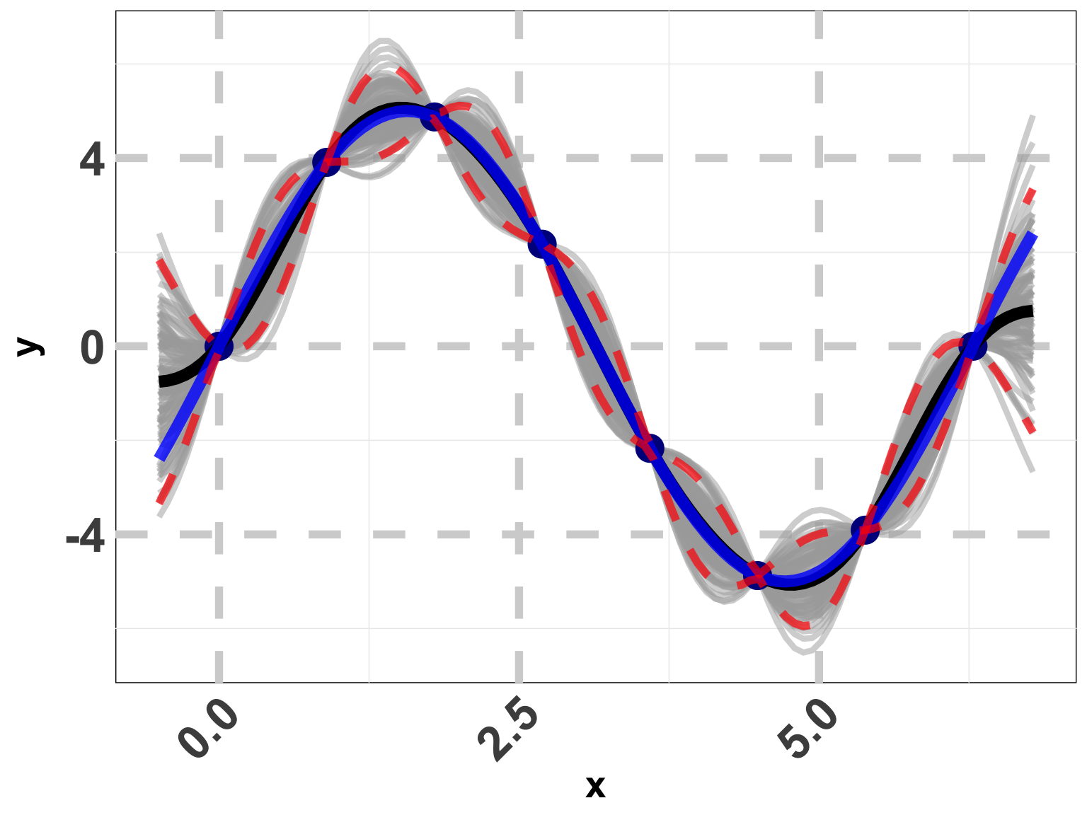
Visualizing a GP

How does a GP work

• Our “fancy” average was just using data around the new location.

• We are using points closer to each other to correlate the responses.

• Now we know, we are averaging the data “nearby”… How do you define that?

• This indicates that we are using distance in some way. Where…? We need some math

Mathematically

• Any normal distribution can be described by a mean vector \mu and a covariance matrix \Sigma.

• Mathematically, we can write it as,

Y_{\ n \times 1} \sim N \ ( \ \mu(X)_{\ n \times 1} \ , \ \Sigma(X)_{ \ n \times n} \ ) Here, Y is the response of interest and n is the number of observations.

• Our goal is to find Y_p \ \vert \ Y, X.

Distance

• Recall that in Linear Regression, you have \ \Sigma \ = \sigma^2 \mathbb{I}

• For a GP, the covariance matrix ( \Sigma ) is defined by a kernel.

• Consider,

\Sigma_n = \tau^2 C_n where C_n = \exp \left( - \vert \vert x - x' \vert \vert^2 \right), and x and x' are input locations.

Interpretation of the kernel

• C_n = \exp \left( - \vert \vert x - x' \vert \vert^2 \right)

• The covariance structure now depends on how close together the inputs. If inputs are close in distance, then the responses are more highly correlated.

• The covariance will decay at an exponential rate as x moves away from x'.

Summarizing our data

• Now we will learn how to use a GP to make predictions at new locations.

• As we learnt, we condition on the data. We can think of this as the prior.

\begin{equation} Y_n \ \vert X_n \sim \mathcal{N} \ ( \ 0 \ , \ \tau^2 \ C_n(X_n) \ ) \\ \end{equation}

Now, consider, (\mathcal{X}, \mathcal{Y}) as the predictive set.

How to make predictions

• The goal is to find the distribution of \mathcal{Y} \ \vert X_n, Y_n which in this case is the posterior distribution.

• By properties of Normal distribution, the posterior is also normally distributed.

We also need to write down the mean and variance of the posterior distribution so it’s ready for use.

How to make predictions

• First we will “stack” the predictions and the data.

\begin{equation*} \begin{bmatrix} \mathcal{Y} \\ Y_n \\ \end{bmatrix} \ \sim \ \mathcal{N} \left( \; \begin{bmatrix} 0 \\ 0 \\ \end{bmatrix}\; , \; \begin{bmatrix} \Sigma(\mathcal{X}, \mathcal{X}) & \Sigma(\mathcal{X}, X_n)\\ \Sigma({X_n, \mathcal{X}}) & \Sigma_n\\ \end{bmatrix} \; \right) \\[5pt] \end{equation*}

• Now, let’s denote the predictive mean with \mu(\mathcal{X}) and predictive variance with \sigma^2(\mathcal{X})

\begin{equation} \begin{aligned} \mathcal{Y} \mid Y_n, X_n \sim N\left(\mu(\mathcal{X}) \ , \ \sigma^2(\mathcal{X})\right) \end{aligned} \end{equation}

Distribution of Interest!

• We will apply the properties of conditional Normal distributions.

\begin{equation*} \begin{aligned} \mu(\mathcal{X}) & = \Sigma(\mathcal{X}, X_n) \Sigma_n^{-1} Y_n \\[10pt] \sigma^2(\mathcal{X}) & = \Sigma(\mathcal{X}, \mathcal{X}) - \Sigma(\mathcal{X}, X_n) \Sigma_n^{-1} \Sigma(X_n, \mathcal{X}) \\ \end{aligned} \end{equation*}

• Everything we do, relies on these equations. Now, let’s learn more about \Sigma

Sigma Matrix

• \Sigma_n = \tau^2 C_n where C_n is our kernel.

• One of the most common kernels which we will focus on is the squared exponential distance kernel written as

C_n = \exp{ \left( -\frac{\vert\vert x - x' \vert \vert ^2}{\theta} \right ) + g \mathbb{I_n}}

• What’s \tau^2, g and \theta though? No more math. We will just conceptually go through these

Hyper Parameters

A GP is non parameteric, however, has some hyper-parameters. In this case,

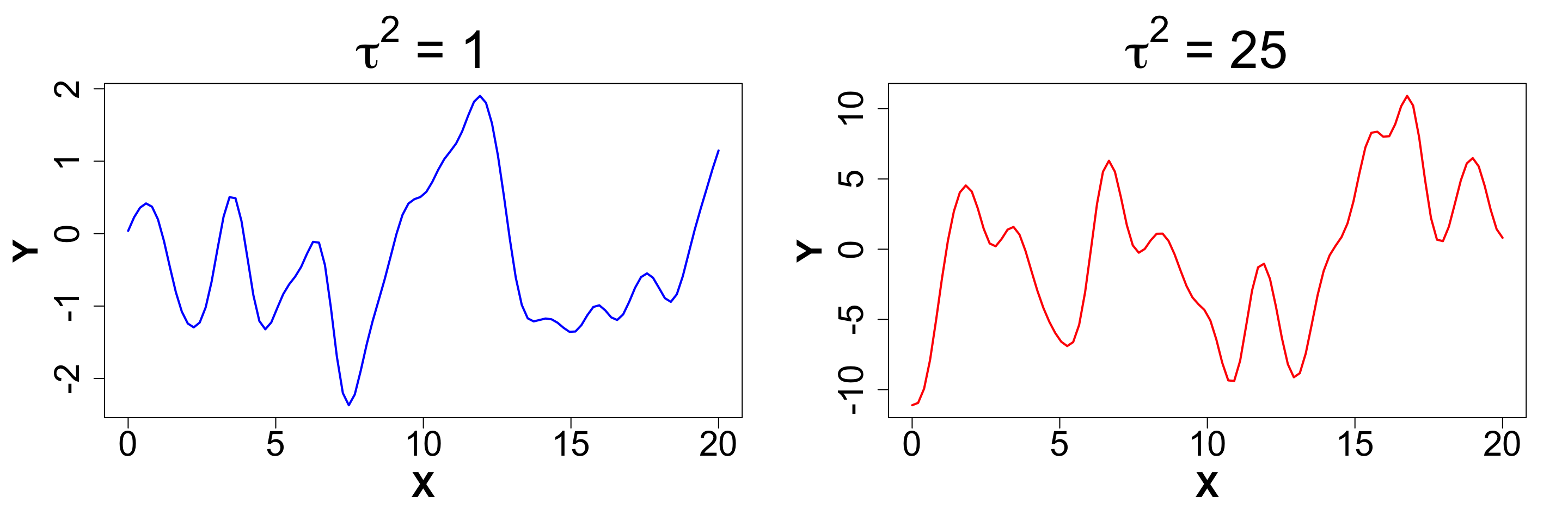
• \tau^2 (Scale): This parameter can be used to adjust the amplitude of the data.

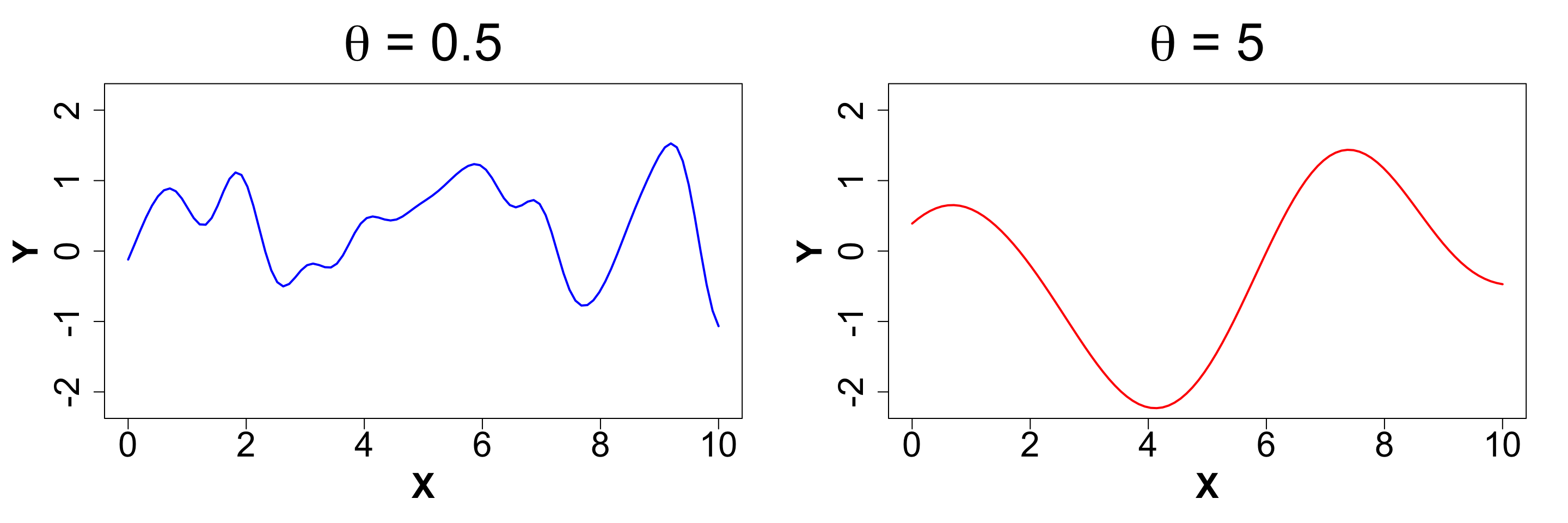
• \theta (Length-scale): This parameter controls the rate of decay of correlation.

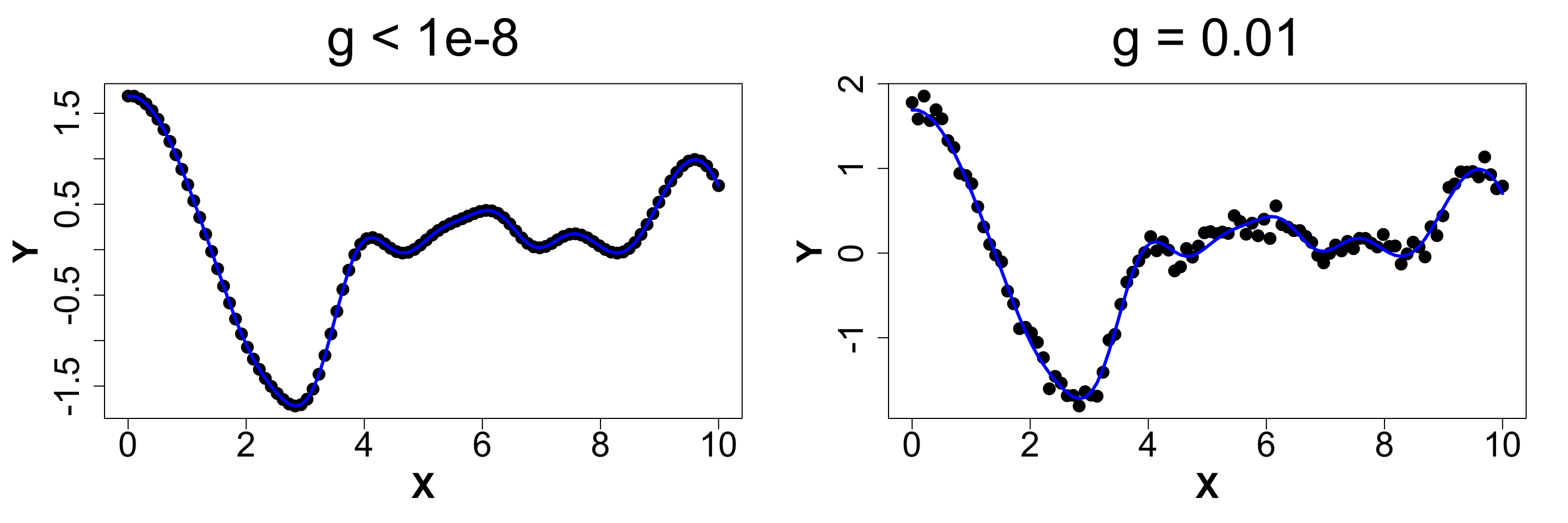
• g (Nugget): This parameter controls the noise in the covariance structure (adds discontinuity)

Scale (Amplitude)

• A random draw from a multivariate normal distribution with \tau^2 = 1 will produce data between -2 and 2.

• Now let’s visualize what happens when we increase \tau^2 to 25.

Length-scale (Rate of decay of correlation)

• Determines how “wiggly” a function is

• Smaller \theta means wigglier functions i.e. visually:

Nugget (Noise)

• Ensures discontinuity and prevents interpolation which in turn yields better UQ.

• We will compare a sample from g ~ 0 (< 1e-8 for numeric stability) vs g = 0.1 to observe what actually happens.

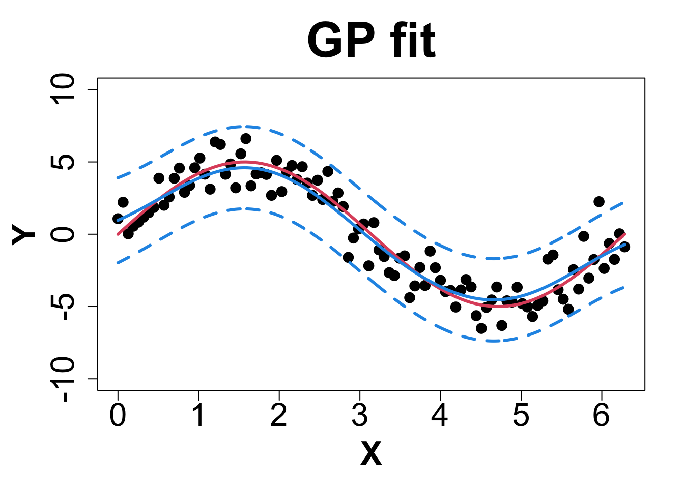
Toy Example (1D Example)

X <- matrix(seq(0, 2*pi, length = 100), ncol =1)
n <- nrow(X) 
true_y <- 5 * sin(X)
obs_y <- true_y + rnorm(n, sd=1)

Toy Example (1D Example)

eps <- sqrt(.Machine$double.eps)
gpi <- laGP::newGP(X = X,Z = obs_y, d = 0.1, g = 0.1 * var(obs_y), dK = TRUE) 
mle <- laGP::mleGP(gpi = gpi, param = c("d", "g"), 
                   tmin= c(eps, eps), tmax= c(10, var(obs_y))) 
XX <- matrix(seq(0, 2*pi, length = 1000), ncol =1)
p <- laGP::predGP(gpi = gpi, XX = XX)

Extentions

• Anisotropic Gaussian Processes: Suppose our data is multi-dimensional, we can control the length-scale (\theta) for each dimension.

• Heteroskedastic Gaussian Processes: Suppose our data is noisy and the noise is input dependent, then we can use a different nugget for each unique input rather than a scalar g.

Anisotropic Gaussian Processes

In this situation, we can rewrite the C_n matrix as,

C_\theta(x , x') = \exp{ \left( -\sum_{k=1}^{m} \frac{ (x_k - x_k')^2 }{\theta_k} \right ) + g \mathbb{I_n}}

Here, \theta = (\theta_1, \theta_2, …, \theta_m) is a vector of length-scales, where m is the dimension of the input space.

Heteroskedastic Gaussian Processes

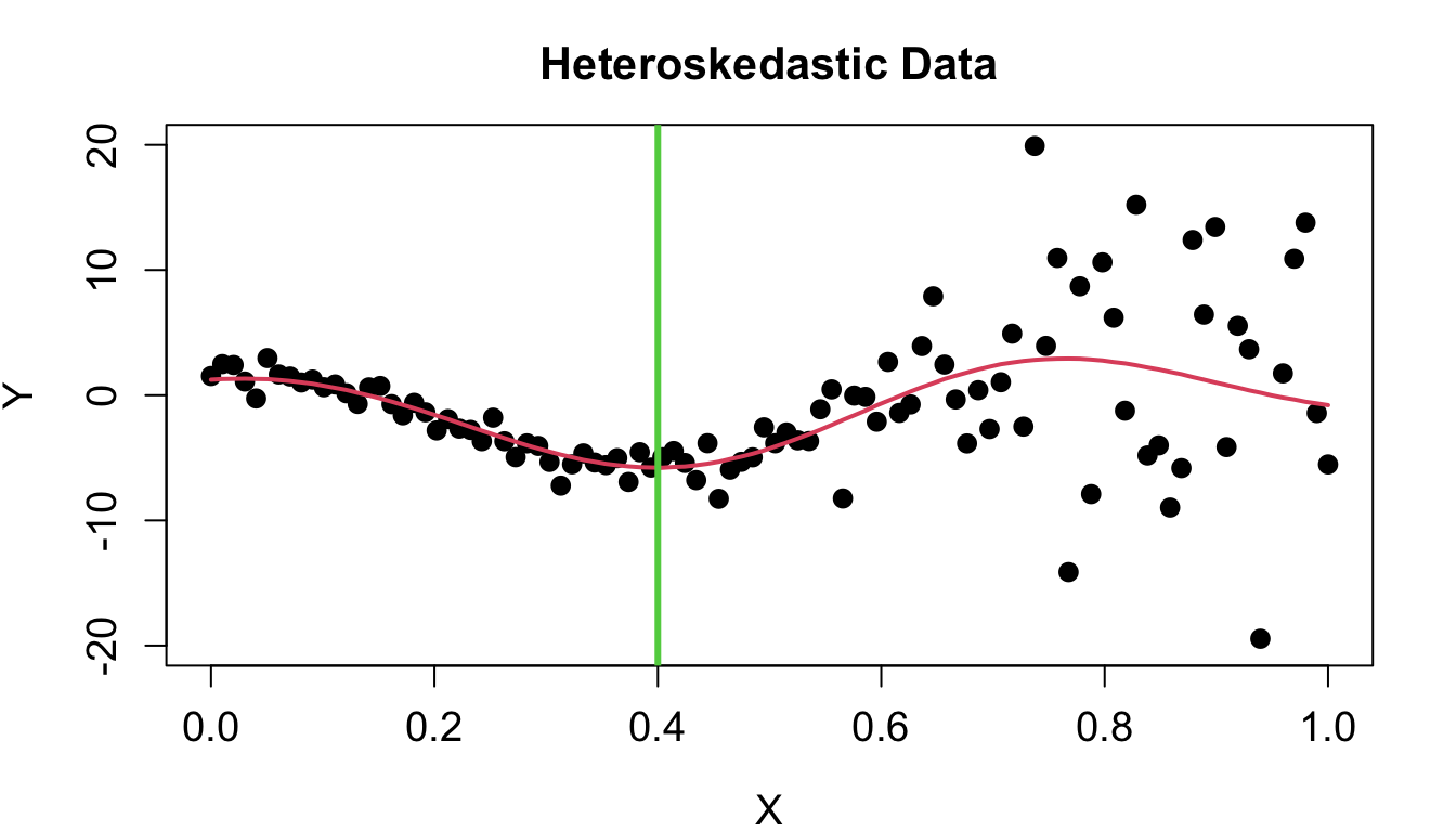
• Heteroskedasticity implies that the data is noisy, and the noise is input dependent and irregular. (Binois, Gramacy, and Ludkovski 2018)

HetGP Setup

• Let Y_n be the response vector of size n. 

• Let X = (X_1, X_2 ... X_n) be the input space.

Then, a regular GP is written as:

\begin{align*} Y_N \ & \ \sim GP \left( 0 \ , \tau^2 C_n \right); \ \text{where, }\\[2pt] C_n & \ = \exp{ \left( -\frac{\vert\vert x - x' \vert \vert ^2}{\theta} \right ) + g \mathbb{I_n}} \end{align*}

HetGP Setup

In case of a hetGP, we have:

\begin{aligned} Y_n\ & \ \sim GP \left( 0 \ , \tau^2 C_{n, \Lambda} \right) \ \ \text{where, }\\[2pt] C_{n, \Lambda} & \ = \exp{ \left( -\frac{\vert\vert x - x' \vert \vert ^2}{\theta} \right ) + \Lambda_n} \ \ \ \text{and, }\ \ \\[2pt] \ \ \Lambda_n \ & \ = \ \text{Diag}(\lambda_1, \lambda_2 ... , \lambda_n) \\[2pt] \end{aligned}

• Instead of one nugget for the GP, we have a vector of nuggets i.e. a unique nugget for each unique input.

HetGP Predictions

• Recall, for a GP, we make predictions using the following:

\begin{equation*} \begin{aligned} \mu(\mathcal{X}) & = \Sigma(\mathcal{X}, X_n) \Sigma_n^{-1} Y_n \\ \sigma^2(\mathcal{X}) & = \Sigma(\mathcal{X}, \mathcal{X}) - \Sigma(\mathcal{X}, X_n) \Sigma_n^{-1} \Sigma(X_n, \mathcal{X}) \\ \end{aligned} \end{equation*}

• We can make predictions using these same equations with \Sigma(X_n) \ \ = \tau^2 C_{n, \Lambda}

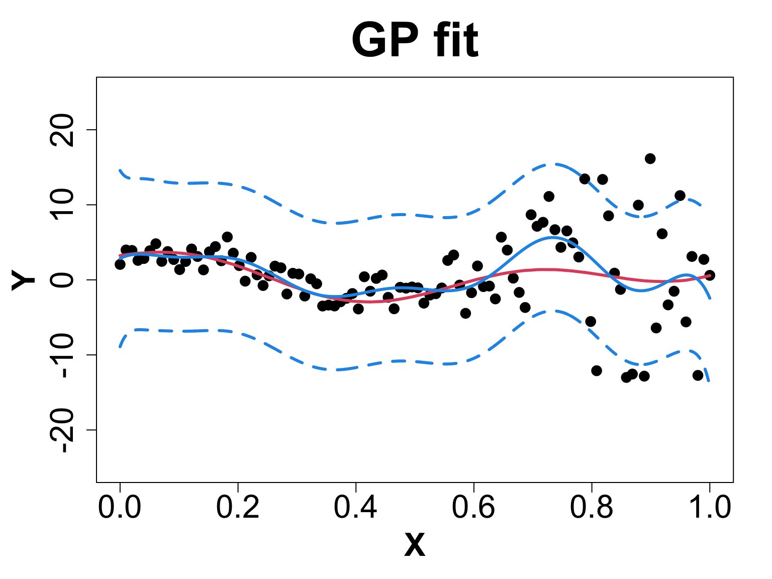
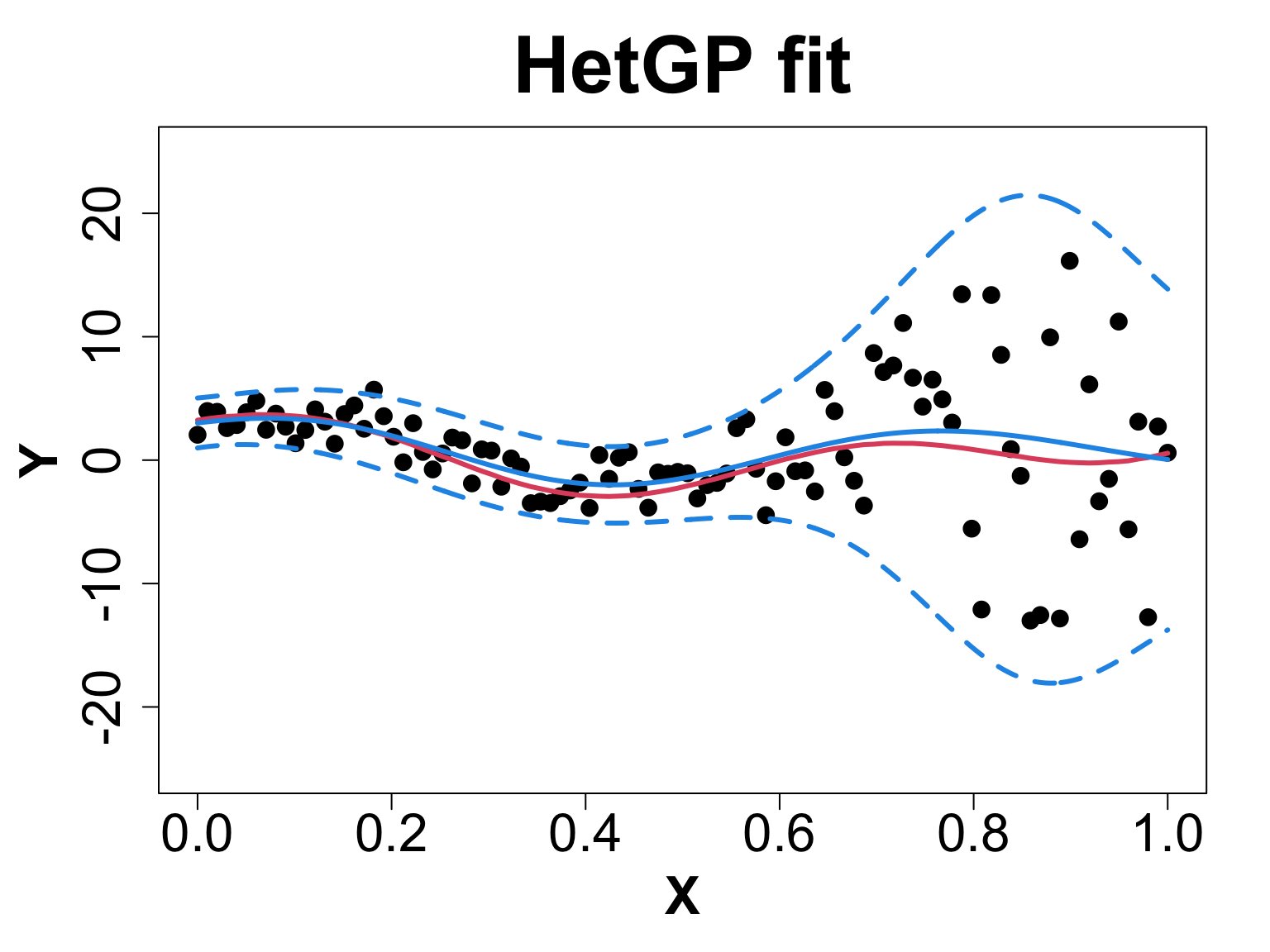
Toy Example (1D Example)

Toy Example (1D Example)

Toy Example (1D Example)

Intro to Ticks Problem

• EFI-RCN held an ecological forecasting challenge NEON Forecasting Challenge (Thomas et al. 2022)

• We focus on the Tick Populations theme which studies the abundance of the lone star tick (Amblyomma americanum)

Tick Population Forecasting

Some details about the challenge:

• Objective: Forecast tick density for 4 weeks into the future

• Sites: The data is collected across 9 different sites, each plot was of size 1600m^2 using a drag cloth

• Data: Sparse and irregularly spaced. We only have ~650 observations across 10 years at 9 locations

Predictors

• X_1 Iso-week: The week in which the tick density was recorded.

• X_2 Sine wave: \left( \text{sin} \ ( \frac{2 \ \pi \ X_1}{106} ) \right)^2.

• X_3 Greenness: Environmental predictor (in practical)

Practical

• Setup these predictors
• Transform the data to normal
• Fit a GP to the Data
• Make Predictions on a testing set
• Check how predictions perform.

References

Binois, Mickael, Robert B Gramacy, and Mike Ludkovski. 2018. “Practical Heteroscedastic Gaussian Process Modeling for Large Simulation Experiments.” Journal of Computational and Graphical Statistics 27 (4): 808–21.

Gramacy, Robert B. 2020. Surrogates: Gaussian Process Modeling, Design, and Optimization for the Applied Sciences. Chapman; Hall/CRC.

Thomas, R Quinn, Carl Boettiger, Cayelan C Carey, Michael C Dietze, Leah R Johnson, Melissa A Kenney, Jason S Mclachlan, et al. 2022. “The NEON Ecological Forecasting Challenge.” Authorea Preprints.