VectorByte Methods Training
Introduction to Modeling Time-Dependent Population Data
Population dynamics of disease
The number of hosts, vectors, pathogens, and infected individuals change over time.
We use models models of various types to: - understand relationships - forecast/predict possible future outcomes
What types of models?

- Focus on describing/quantifying patterns
- Statistical Models, e.g. regression, time series
- Seek to understand mechanisms, less prediction
- ODEs, dynamical systems, Stochastic DEs, Individual Based Models
We’ll focus on the tactical end of things here (i.e., no dif eqs)
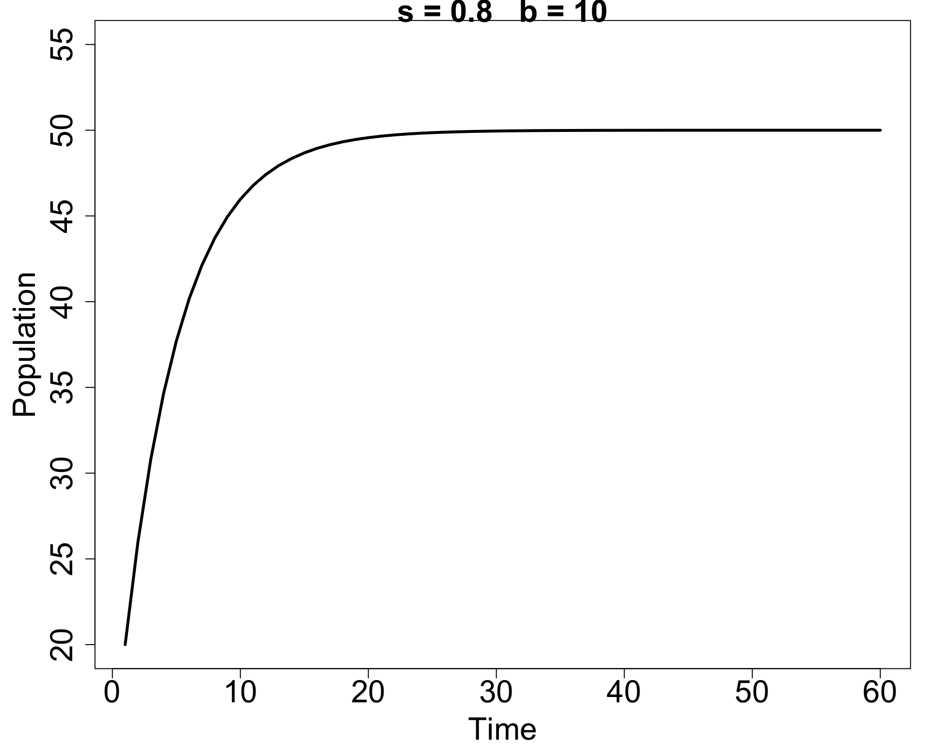
Simple example: A first (deterministic) model
Suppose we model a population in discrete time as \[\begin{align*} N(t+1) = s N(t) + b(t). \end{align*}\]
Here \(s\) is the fraction of individuals surviving each time step and \(b(t)\) is the number of new births.
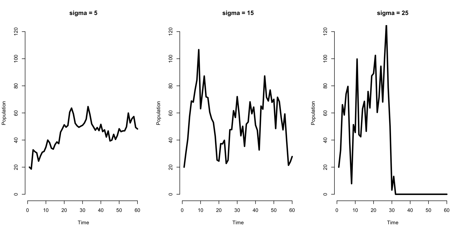
A first (stochastic) model
In that simplest model the population can’t go extinct!
What if the number of births vary? \[\begin{align*} N(t+1) = s N(t) + b(t) +W(t) \end{align*}\]
Here \(W(t)\) is process uncertainty/stochasticity: we assume it is drawn from a particular distribution, and each year/time we observe a particular value \(w(t)\). E.g., \(W(t) \stackrel{\mathrm{iid}}{\sim} \mathcal{N}(0, \sigma^2)\).
What might we see? When would the population go extinct?

Observation Models
We also have to go out into the field and take some observations of the populations.
Let’s say that we observe \(N_{\mathrm{obs}}(t)\) individuals at time \(t\). How does this relate to the true population size? One possibility is: \[\begin{align*} N_{\mathrm{obs}}(t) = N(t) + V(t) \end{align*}\] where \(V(t)\) is our “observation uncertainty”, and all together this equation describes our observation model.
With the observation model, our full system (process + observation models) might be \[\begin{align*} N(t) & = s N(t-1) + b(t-1) +W(t)\\ N_{\mathrm{obs}}(t) & = N(t) + V(t) \end{align*}\]
plus:
- distributions for \(W(t)\), \(V(t)\)
- the initial population size.
Observation process matters
Analysis approach depends on not only the goal of the modeling exercise (understanding vs forecasting/prediction) but also on details of the way that data are observed
- evenly or unevenly spaced observations
- consistent sampling locations
- types of observation/instrument (automated? trap type?)
Although we focus on tools this week, we’ll also talk about general modeling considerations and how to think some of these as we conduct an analyses.
Outline of Course
- Introductions and Goals
- Regression refresher focusing on diagnostics and transformations
- Regression approaches for time dependent data – basics plus time dependent predictors, transformations, simple AR
- Analysis of evenly-spaced data: basic time-series methods
- Abundance data from VecDyn and NEON + climate and meteorological variables
- Advanced modeling with Gaussian Process Models