VectorByte Methods Training: Regression Diagnostics and Transformations (practical)

Author

Affiliation

Leah R. Johnson

Virginia Tech and VectorByte

Overview and Instructions

The goals of this practical are to:

1. Practice building residual diagnostic plots for determining violations of SLR assumptions.
2. Practice matching violations with remedies/transformations evaluating resulting residuals for models fit to transformed data.

Practicing diagnostics and transformations

The file transforms.csv on the course website contains 4 pairs of Xs and Ys. The {\sf R} code from lecture 5B will also be very helpful.

For each pair:

1. Fit the linear regression model Y = \beta_0 + \beta_1 X + \varepsilon, \varepsilon \sim \mathrm{N}(0,\sigma^2). Plot the data and fitted line.

2. Provide a scatterplot, normal Q-Q plot, and histogram for the studentized regression residuals.

3. Using the residual scatterplots, state how the SLR model assumptions are violated.

4. Determine the data transformation to correct the problems in 3, fit the corresponding regression model, and plot the transformed data with new fitted line.

5. Provide plots to show that your transformations have (mostly) fixed the model violations.

Example: Data set 1

Here we take you through an example of analyzing the first of the 4 datasets. You will then use this to practice for the other three.

First we’ll read all of the data in here. You will likely need to change the path to correspond to where your data are stored.

attach(D <- read.csv("data/transforms.csv"))

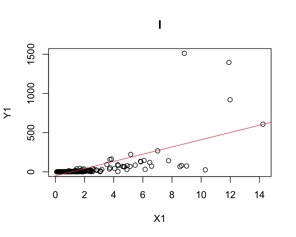
1. Fit the linear regression model. Plot the data and fitted line.

## fit models
lm1 <- lm(Y1 ~ X1)

## plot points and fitted lines
plot(X1, Y1, col=1, main="I"); abline(lm1, col=2)

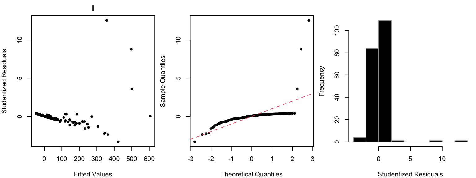
2. Provide a scatterplot, normal Q-Q plot, and histogram for the studentized regression residuals.

par(mfrow=c(1,3), mar=c(4,4,2,0.5))   

## studentized residuals vs fitted
plot(lm1$fitted, rstudent(lm1), col=1,
     xlab="Fitted Values", 
     ylab="Studentized Residuals", 
     pch=20, main="I")

## qq plot of studentized residuals
qqnorm(rstudent(lm1), pch=20, col=1, main="" )
abline(a=0,b=1,lty=2, col=2)

## histogram of studentized residuals
hist(rstudent(lm1), col=1, 
     xlab="Studentized Residuals", 
     main="", border=8)

3. Using the residual scatterplots, state how the SLR model assumptions are violated.

Xs are clumpy AND the variance seems non-constant. It looks a lot like the GDP data from class. Since both Xs and Ys are strictly positive, we can try a log-log transform.

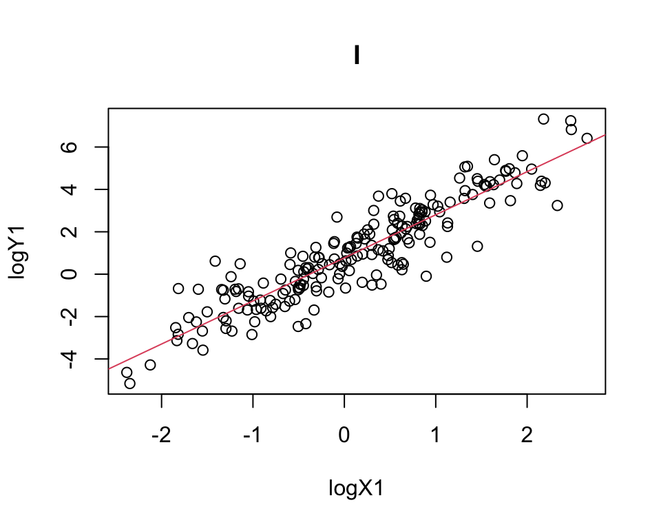
4. Determine the data transformation to correct the problems in 3, fit the corresponding regression model, and plot the transformed data with new fitted line.

### the fix is as follows:
logX1<- log(X1)
logY1 <- log(Y1)

### re-run the regressions and residual plots to show this worked
lm1 <- lm(logY1 ~ logX1)

## plot points and lines
plot(logX1, logY1, col=1, main="I"); abline(lm1, col=2)

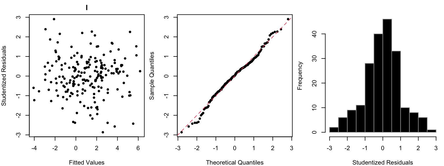
5. Provide plots to show that your transformations have (mostly) fixed the model violations.

## studentized residuals vs fitted

par(mfrow=c(1,3), mar=c(4,4,2,0.5))  
plot(lm1$fitted, rstudent(lm1), col=1,
     xlab="Fitted Values", 
     ylab="Studentized Residuals", 
     pch=20, main="I")

## Q-Q plots
qqnorm(rstudent(lm1), pch=20, col=1, main="" )
abline(a=0,b=1,lty=2, col=2)

## histograms of studentized residuals
hist(rstudent(lm1), col=1, 
     xlab="Studentized Residuals", 
     main="", border=8)

This is much better! The histogram still maybe looks a little funny, but given that the qq-plot looks pretty good, I think we’ve made a good transformation.

Your Turn!

Repeat this process with the other 3 datasets, and see if you can figure out a appropriate transformations for each dataset.