Introduction to Gaussian Processes for Time Dependent Data
Virginia Tech
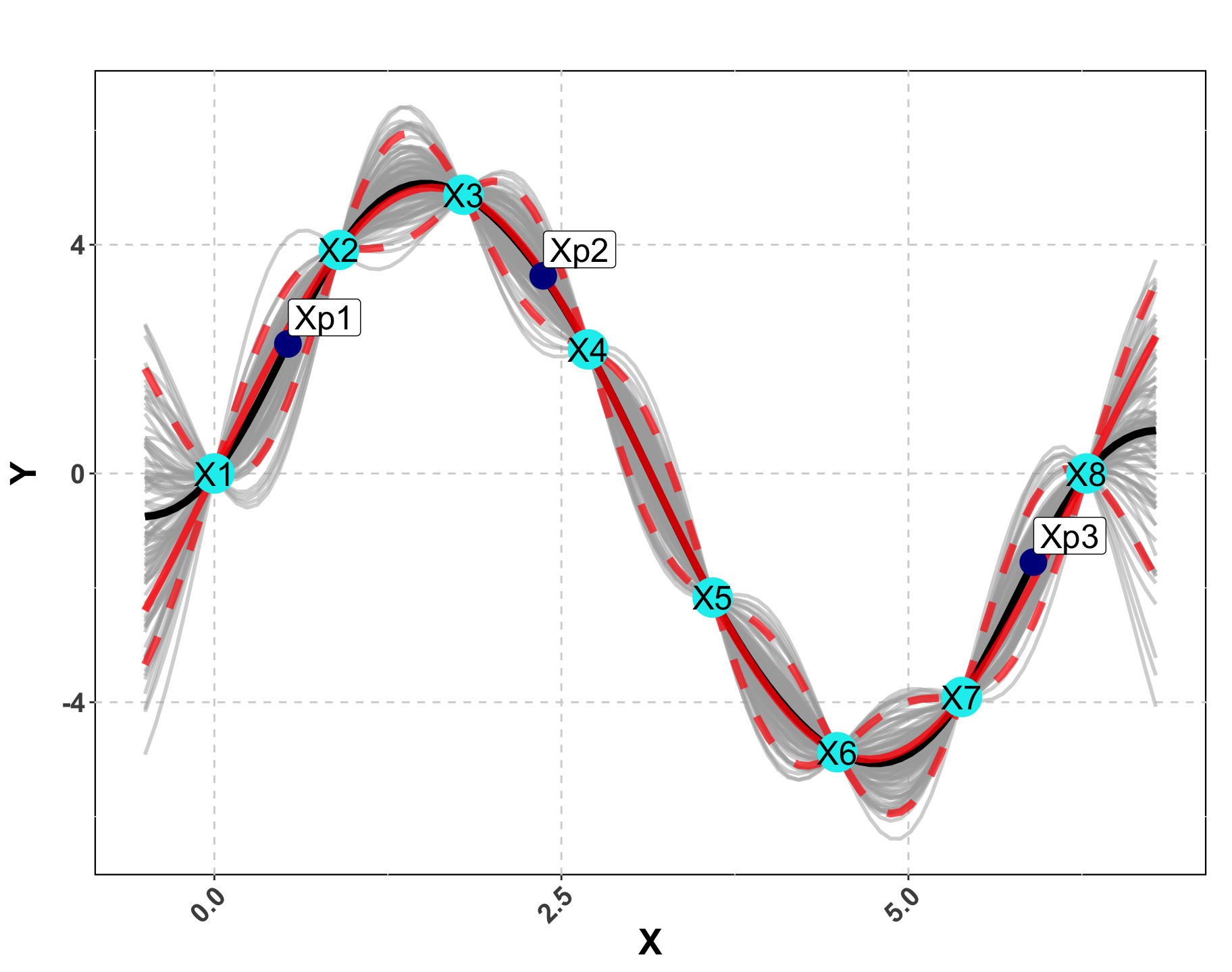
Visualizing a GP
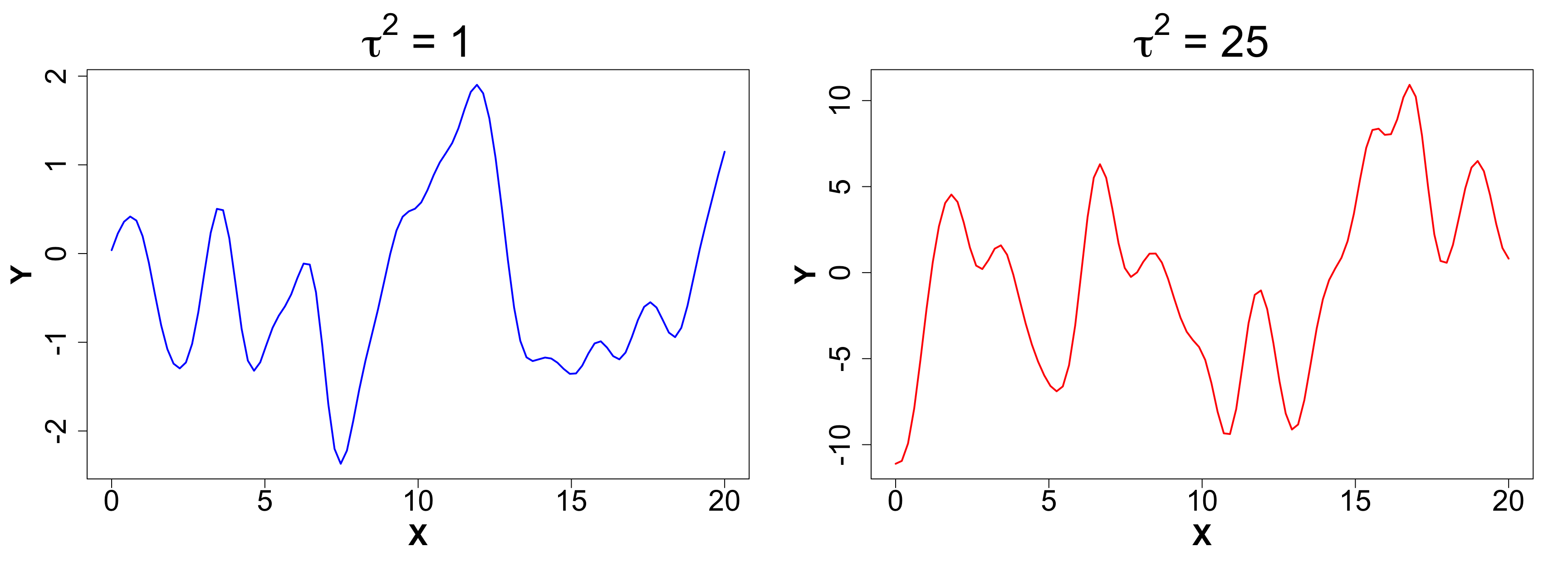
Scale (Amplitude)
A random draw from a multivariate normal distribution with \tau^2 = 1 will produce data between -2 and 2.
Now let’s visualize what happens when we increase \tau^2 to 25.
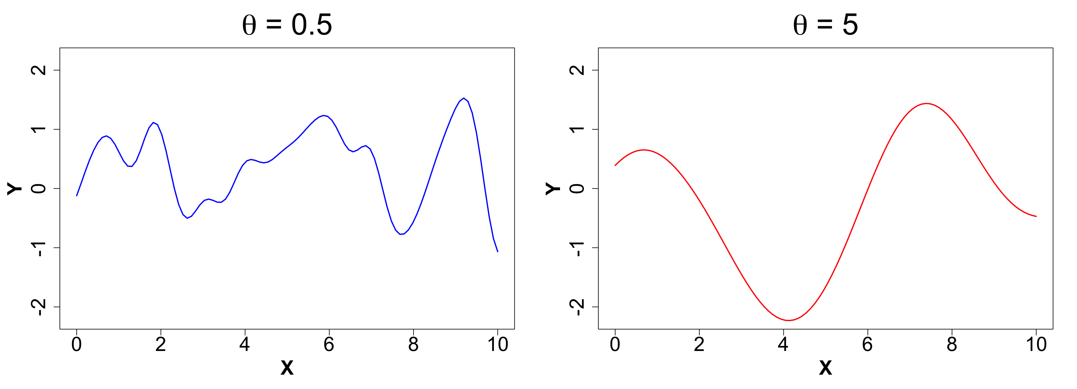
Length-scale (Rate of decay of correlation)
Determines how “wiggly” a function is
Smaller \theta means wigglier functions i.e. visually:
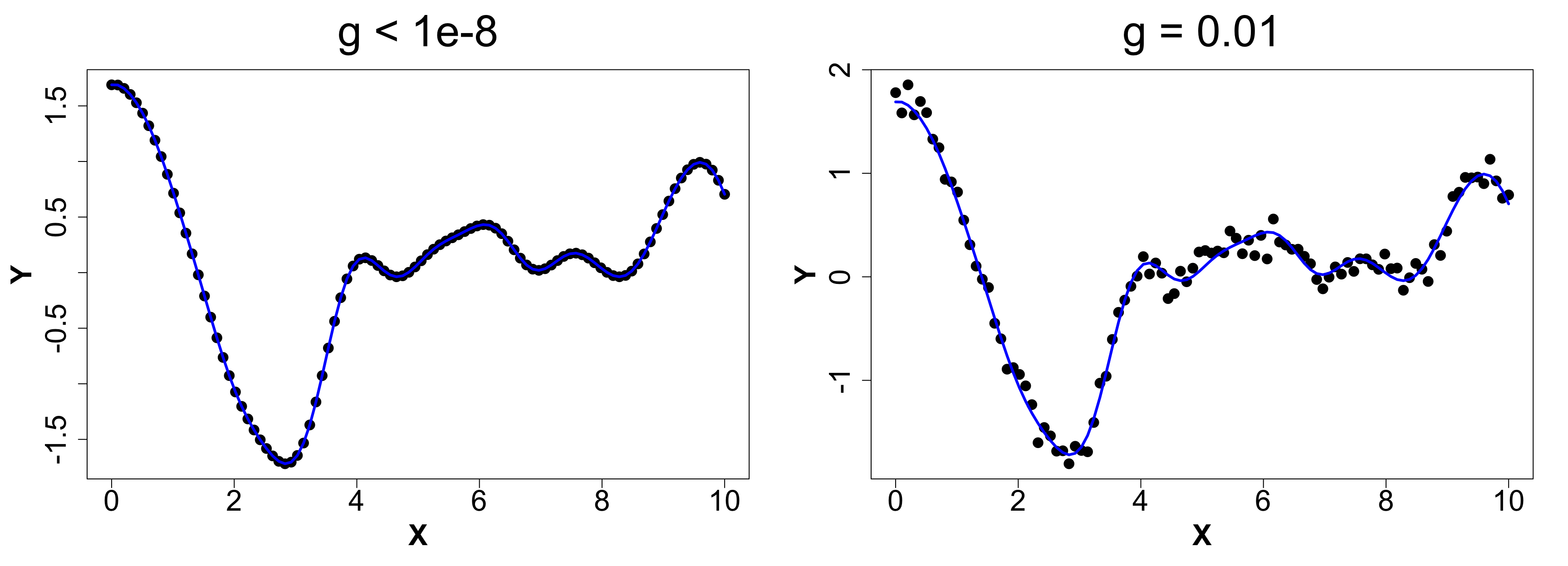
Nugget (Noise)
Ensures discontinuity and prevents interpolation which in turn yields better UQ.
We will compare a sample from g ~ 0 (< 1e-8 for numeric stability) vs g = 0.1 to observe what actually happens.
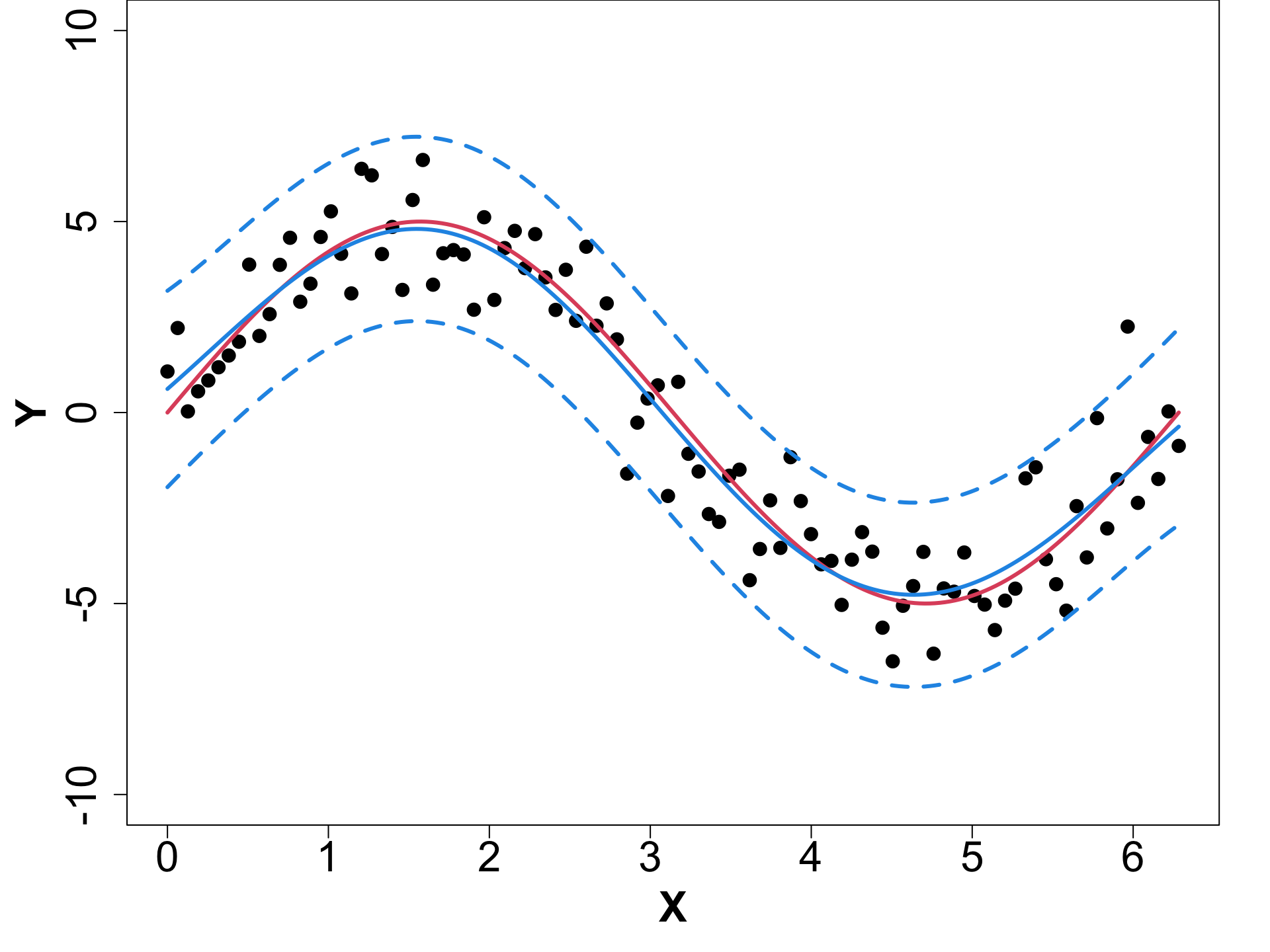
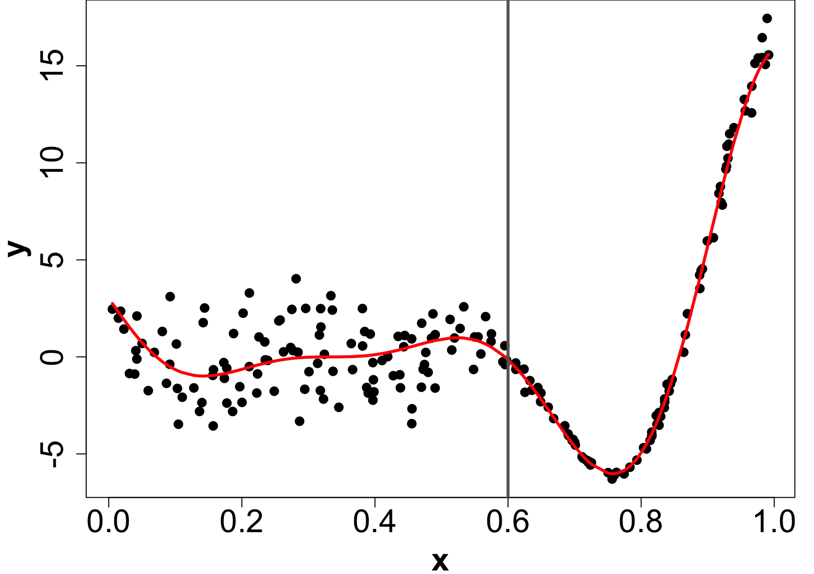
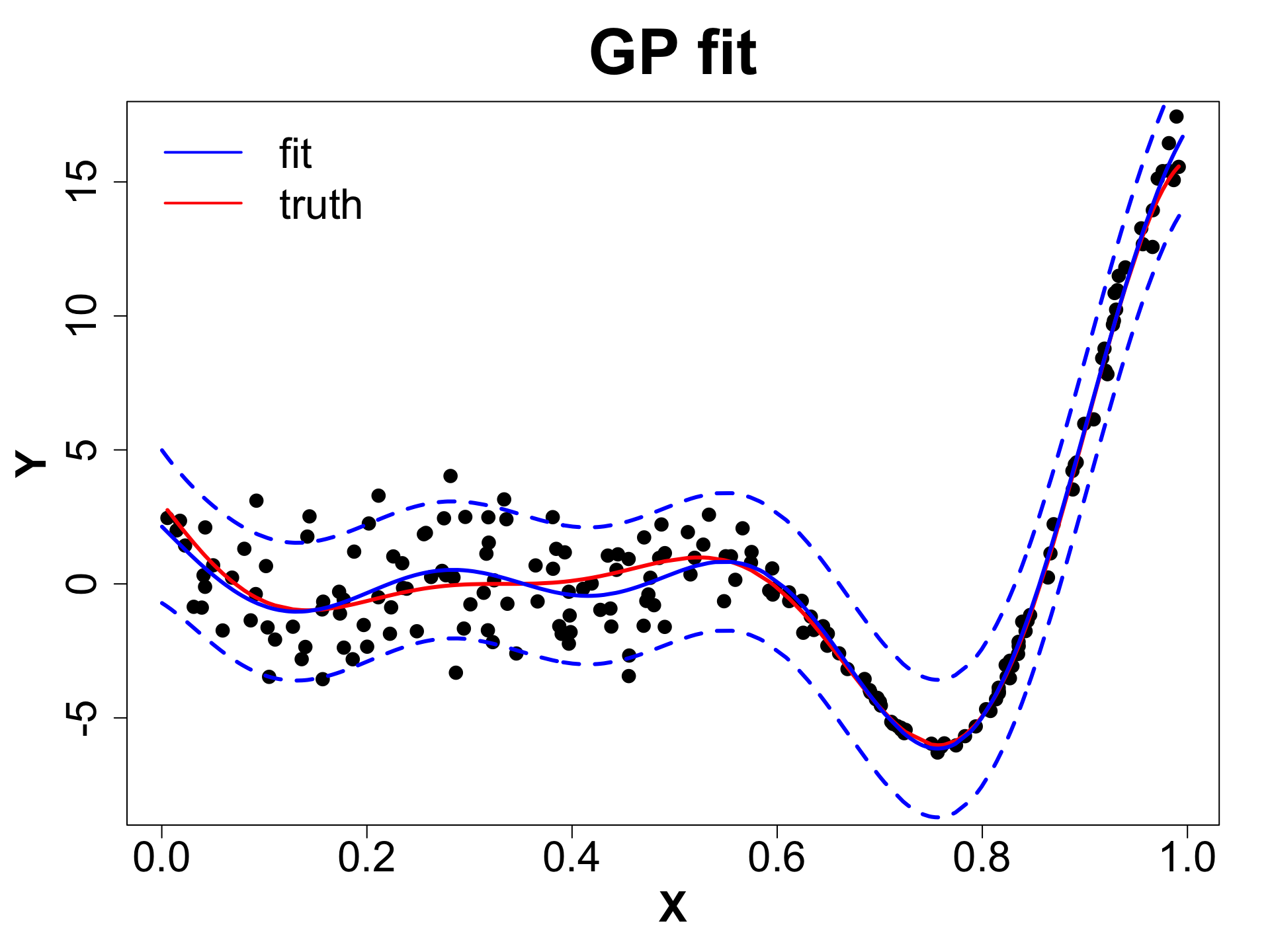
Toy Example (1D Example)
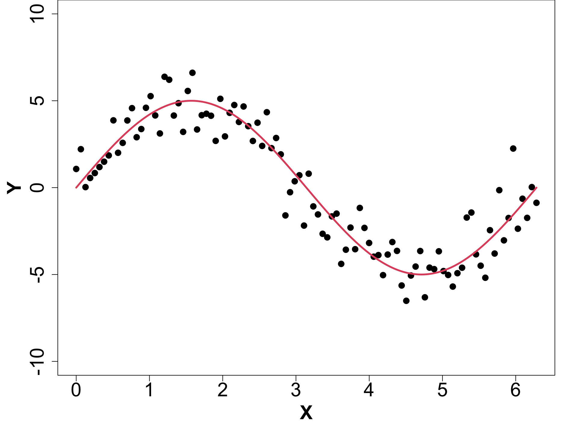
Toy Example (1D Example)

Toy Example (1D Example)
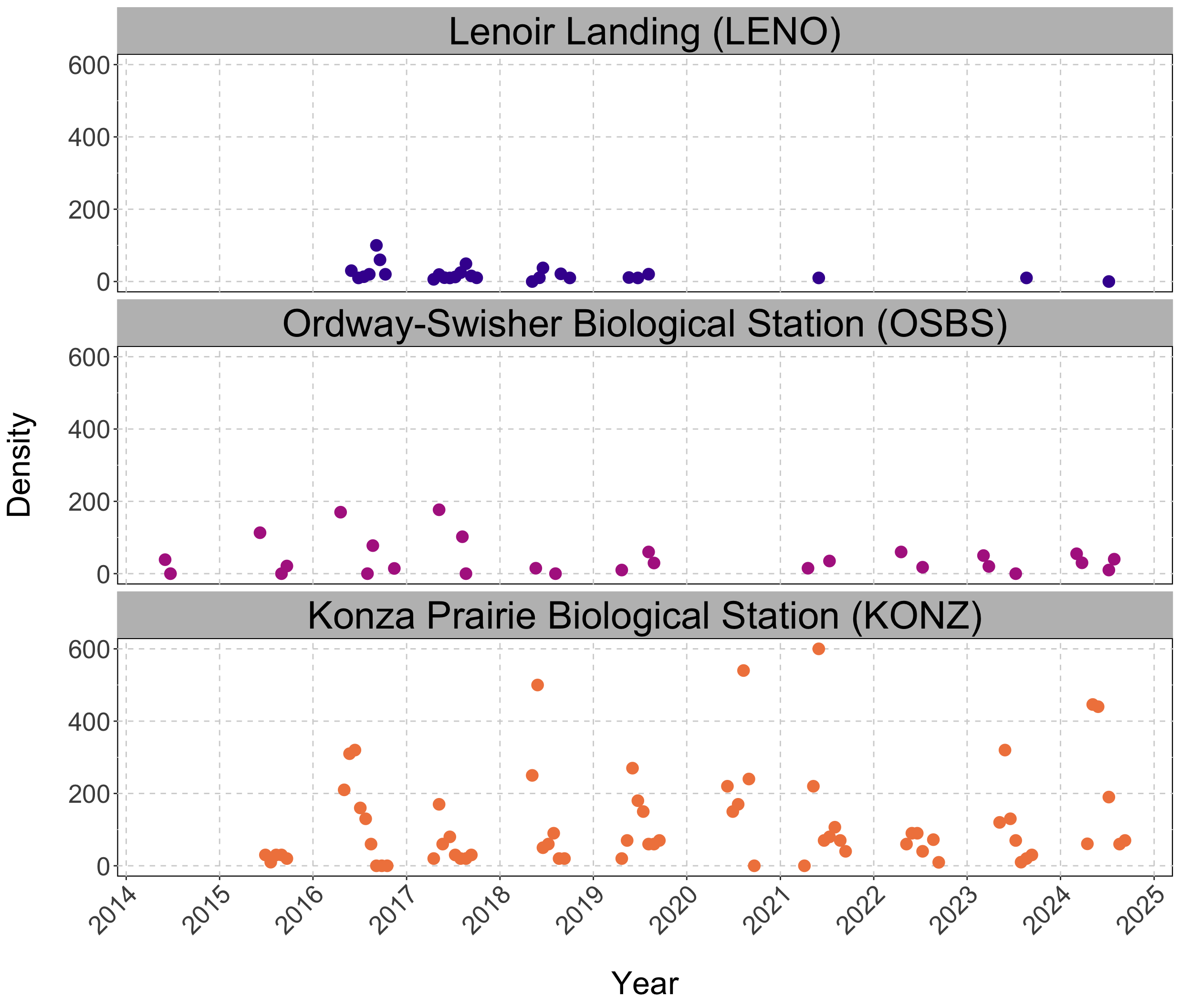
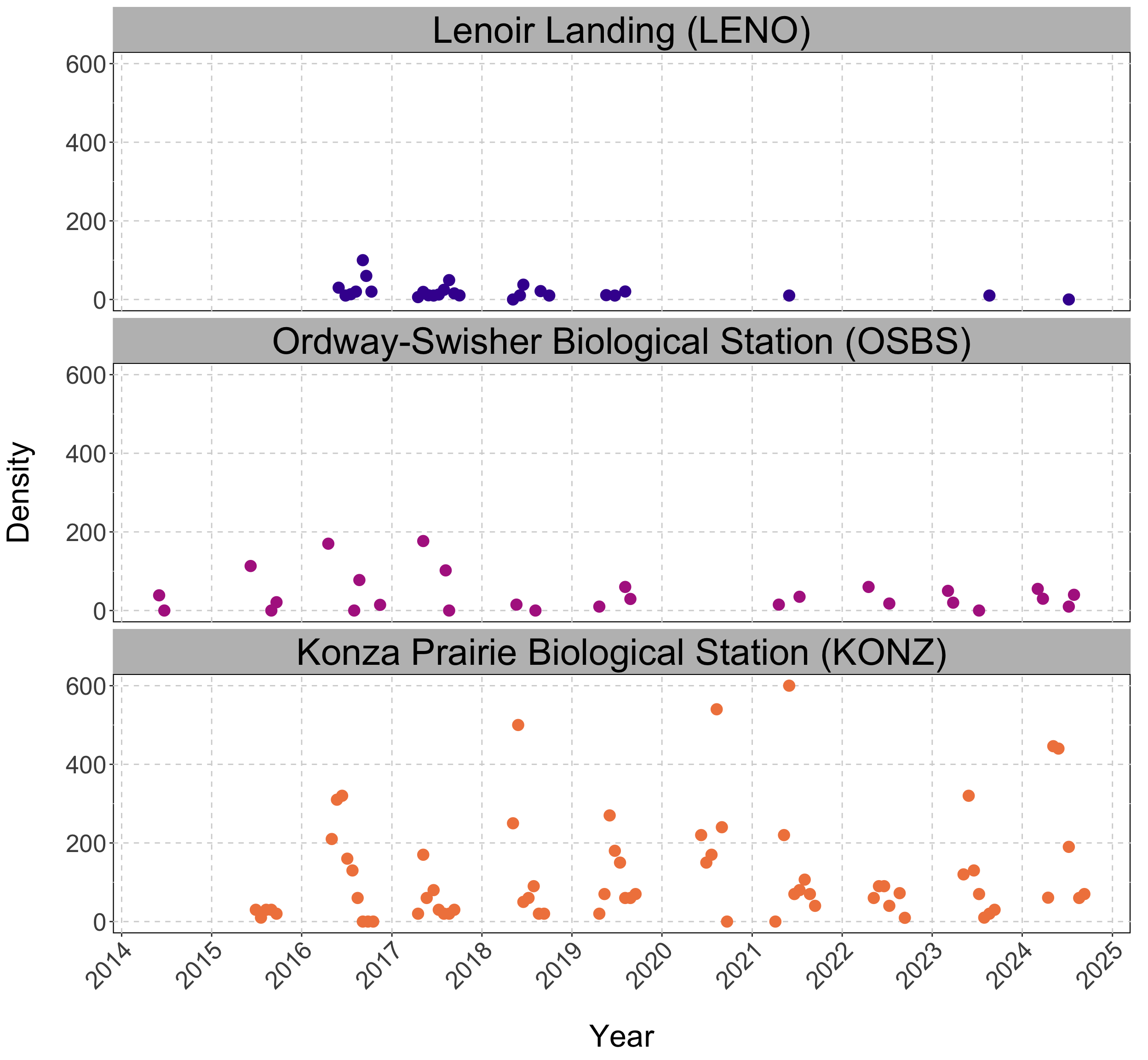
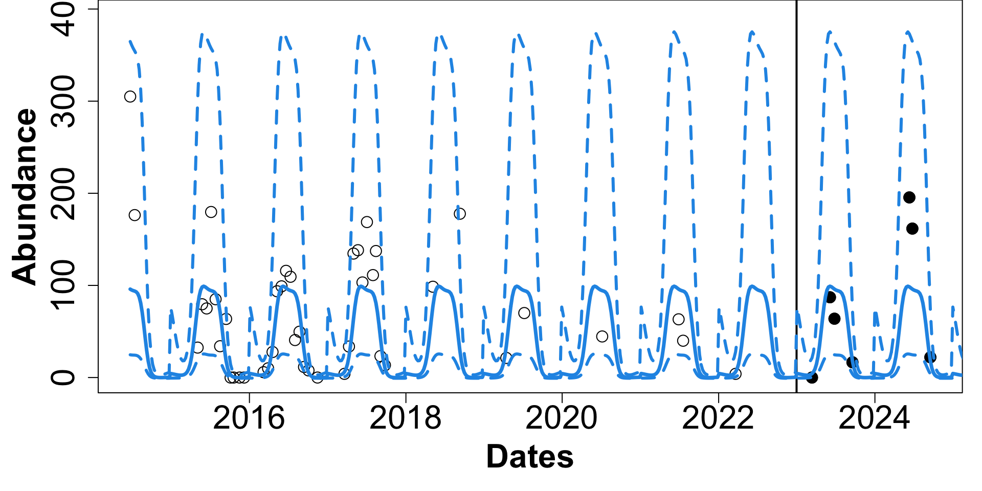
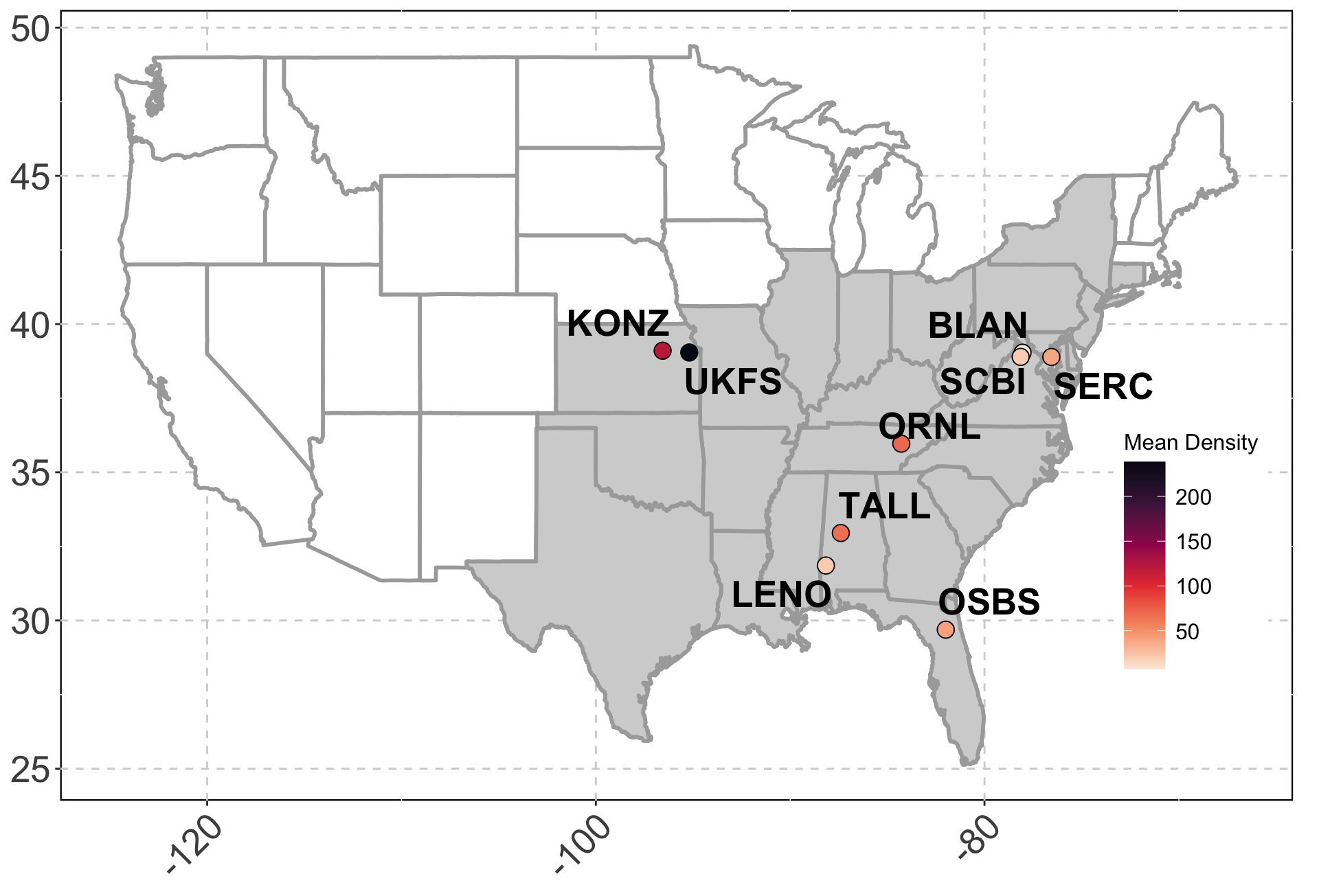
Tick Populations: ORNL
| Iso-week (c) | Periodicity | Transformed Density | |
|---|---|---|---|
| 2014-06-23 | 0.49 | 1.00 | 5.72 |
| 2014-07-14 | 0.55 | 0.98 | 5.18 |
| 2015-05-04 | 0.36 | 0.82 | 3.51 |
Extension: Heteroskedastic GPs (HetGP)
- Suppose we have noise is input dependent (Binois, Gramacy, and Ludkovski 2018).
Extension: Heteroskedastic GPs (HetGP)
- Suppose we have noise is input dependent (Binois, Gramacy, and Ludkovski 2018).

- We can use a different nugget for each unique input rather than a scalar g.
HetGP Predictions
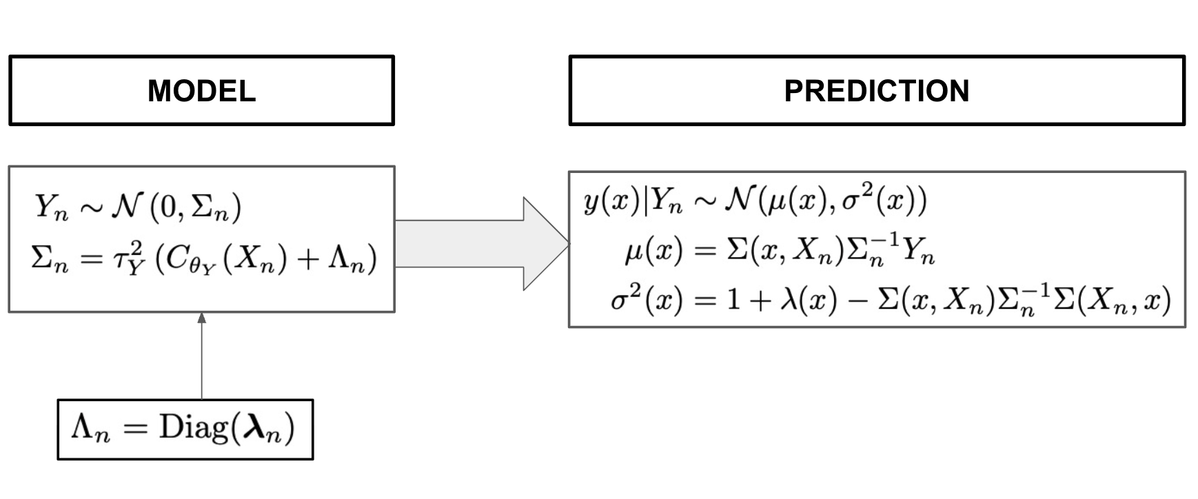
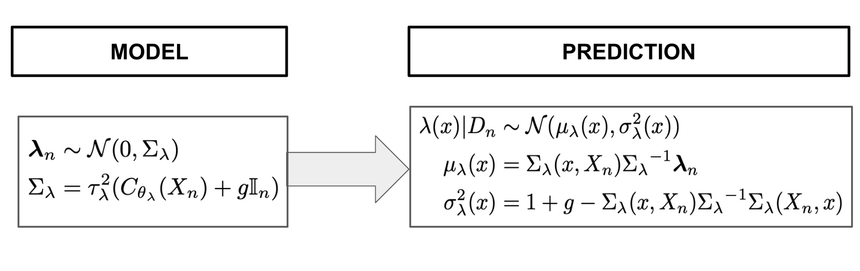
HetGP Latent Layer Modeling
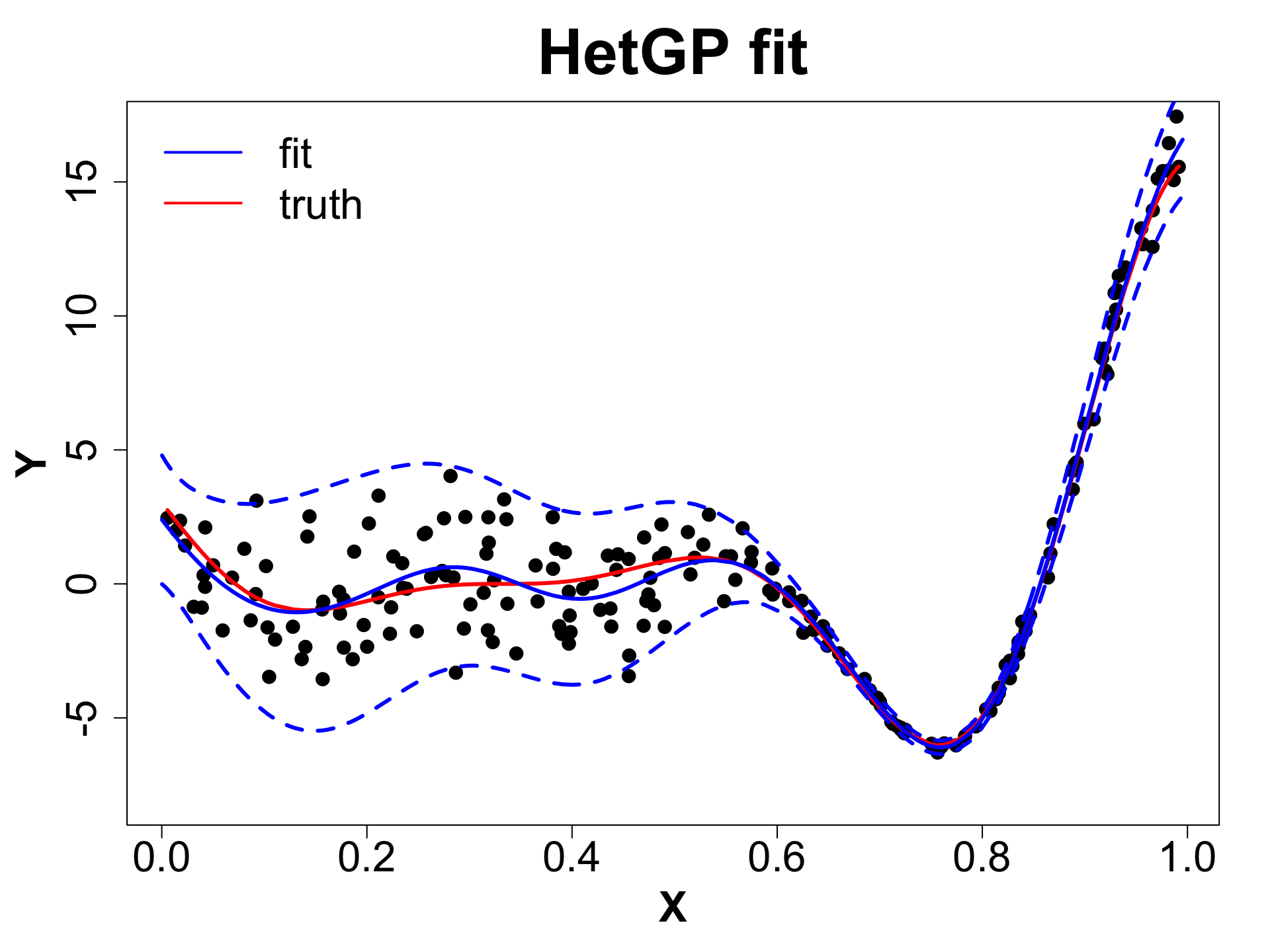
HetGP: Toy Example (1D Example)
HetGP: Toy Example (1D Example)

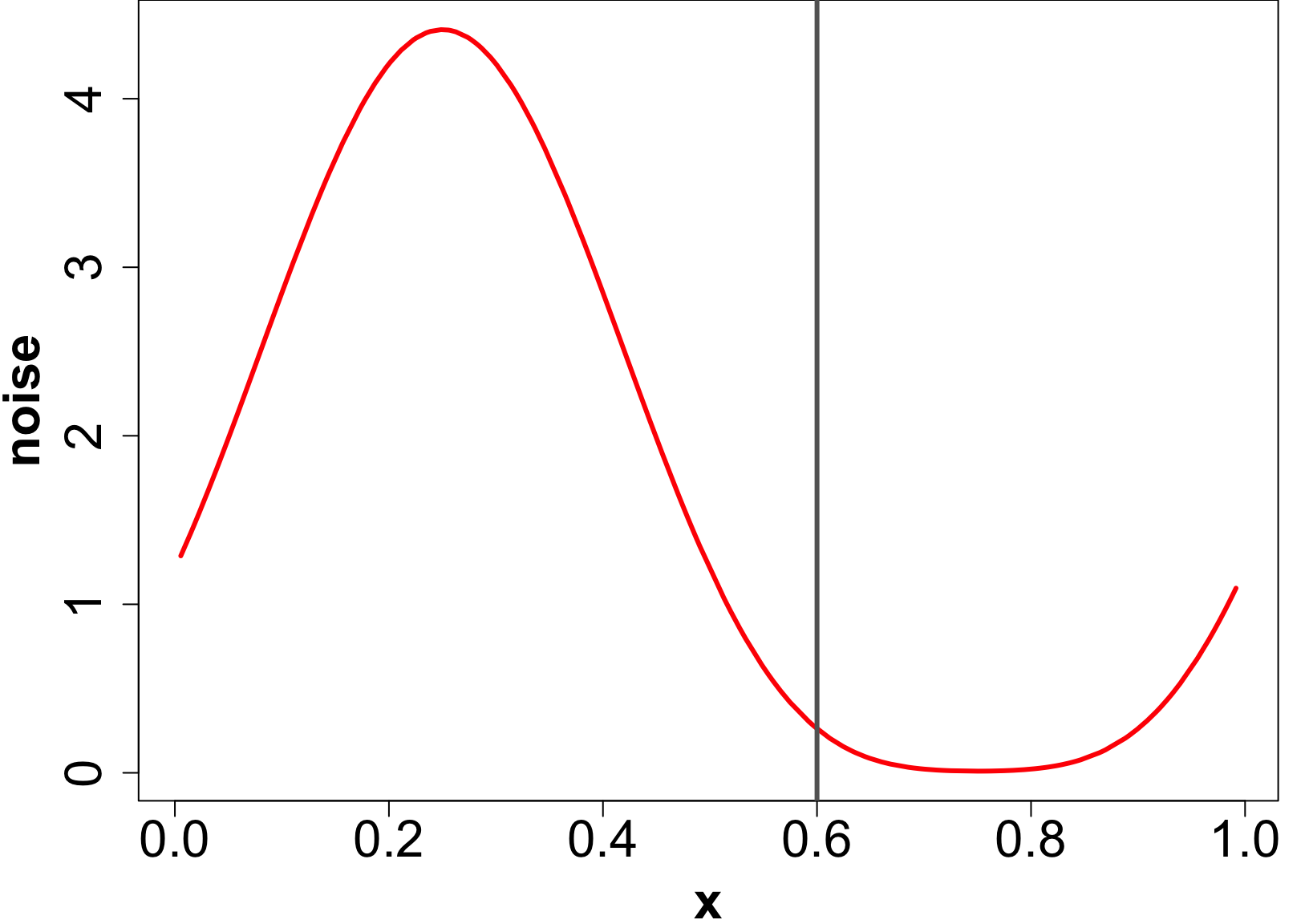
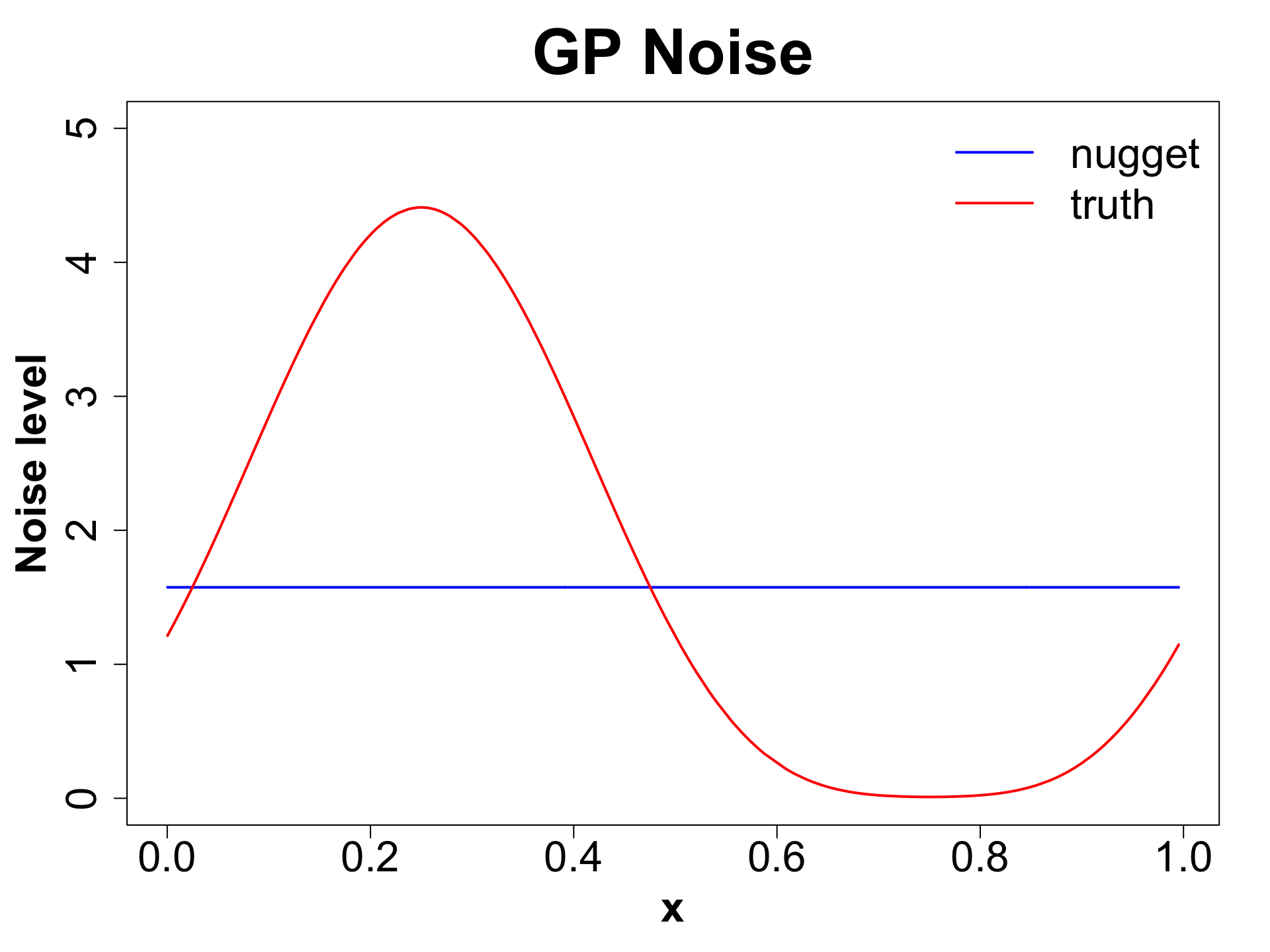
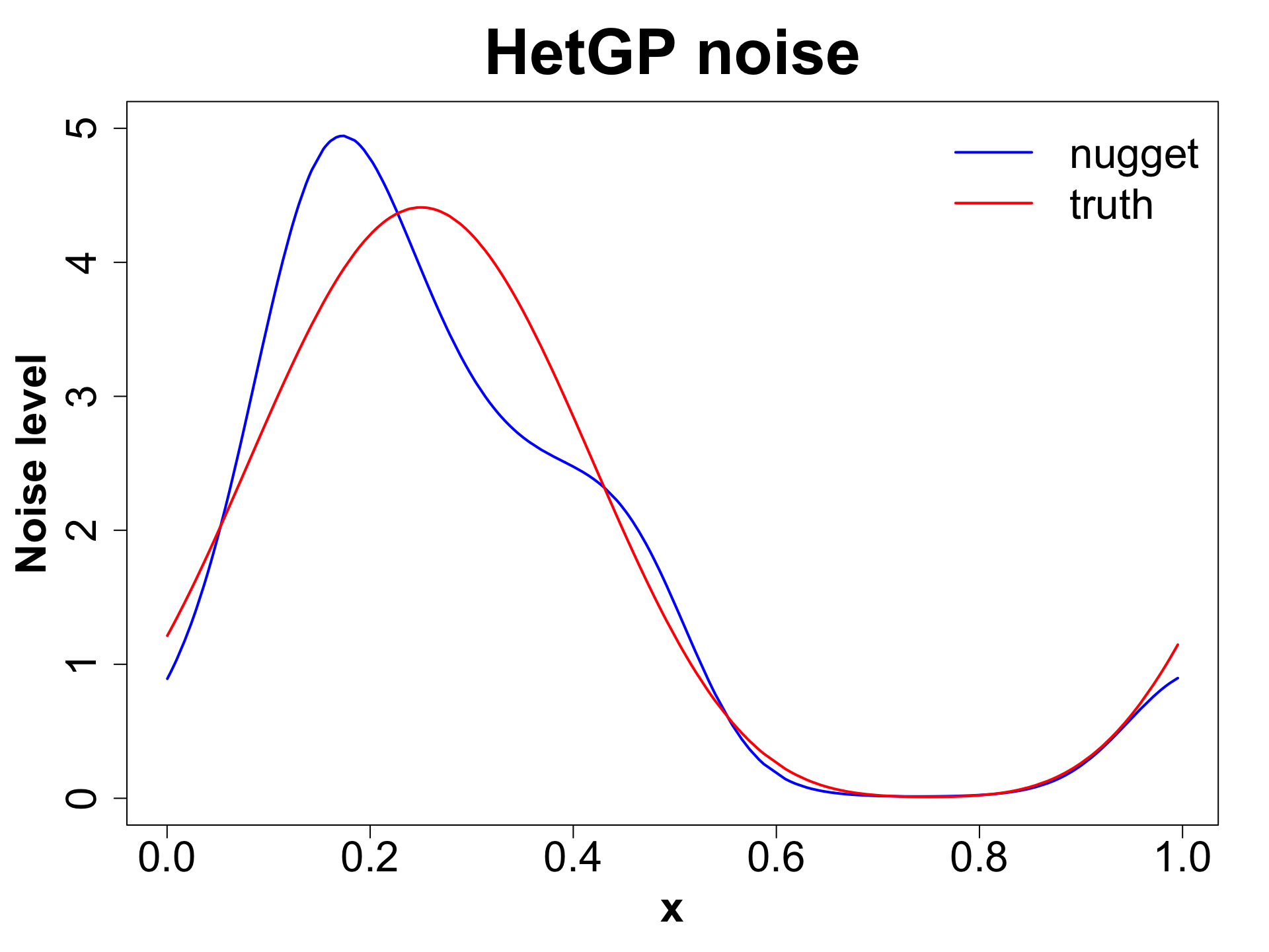
HetGP: Noise Levels
Tick Population Forecasting
EFI-RCN held an ecological forecasting challenge NEON Forecasting Challenge (Thomas et al. 2022)
We focus on the Tick Populations theme which studies the abundance of the lone star tick (Amblyomma americanum)
Objective: Forecast tick density for 4 weeks into the future.
Sites: The data is collected across 9 different NEON plots.
Data: Sparse and irregularly spaced.
n = ~570 observations since 2014.
Predictors
Iso-week, X_1 = 1,2,... 53.
Periodicity, X_2 = \text{sin}^2 \left( \frac{2 \pi X_1}{106} \right).
Mean Elevation, X_3.