The VectorByte Team (Leah R. Johnson and Alicia Arneson, Virginia Tech)
Learning Objectives
Introduce traditional time-series approaches
Be able to conduct simple time series analyses
Be able to produce a forecast for a time series model.
Recall: Time Series Data
Time dependent data may be considered a comprise a time series (TS) if the data are observed at evenly spaced intervals.
Most TS methods WILL NOT work properly if data are irregularly spaced
Occasionally data points may be missing – then there are methods to interpolate.
Irregularly spaced data may be aggregated in a systematic way to fulfill the TS requirements.
Components of a time-series model
We can classify the patterns that we wish to quantify with a time series model into five categories:
Level: the average value of the overall TS
Trend: whether the TS tends to go up or down
Seasonality: the tendency of the TS to repeat or cycle with a set frequency
Auto-regression: correlation in the TS with nearby times
Noise: random components, not correlated to other parts of the model
Last time: Regression based
We previously used a regression approach to allow us to explore these patterns:
Level: usually the intercept in the model
Trend: added time as a predictor
Seasonality: included sine/cosine predictors
Auto-regression: response at lagged times as a predictor
Noise: assumed additive, normal noise
We want to expand our toolbox and give ourselves more options to build models, and eventually use them to forecast!.
First approach – Smoothing
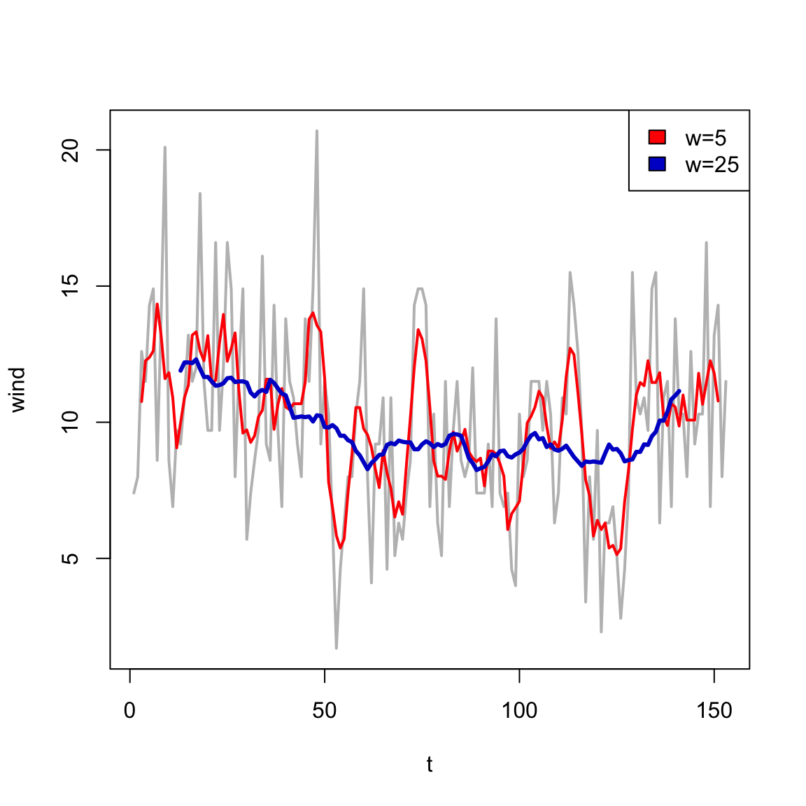
Often one of the first things we want to do is smooth a TS. This is simply averaging multiple time periods to reduce noise.
This can, on it’s own, bring out the “signal” in a TS.
It’s also super useful to produce smoothed time dependent predictors, so that you’re not using noise/extreme values to predict patterns in your target TS.
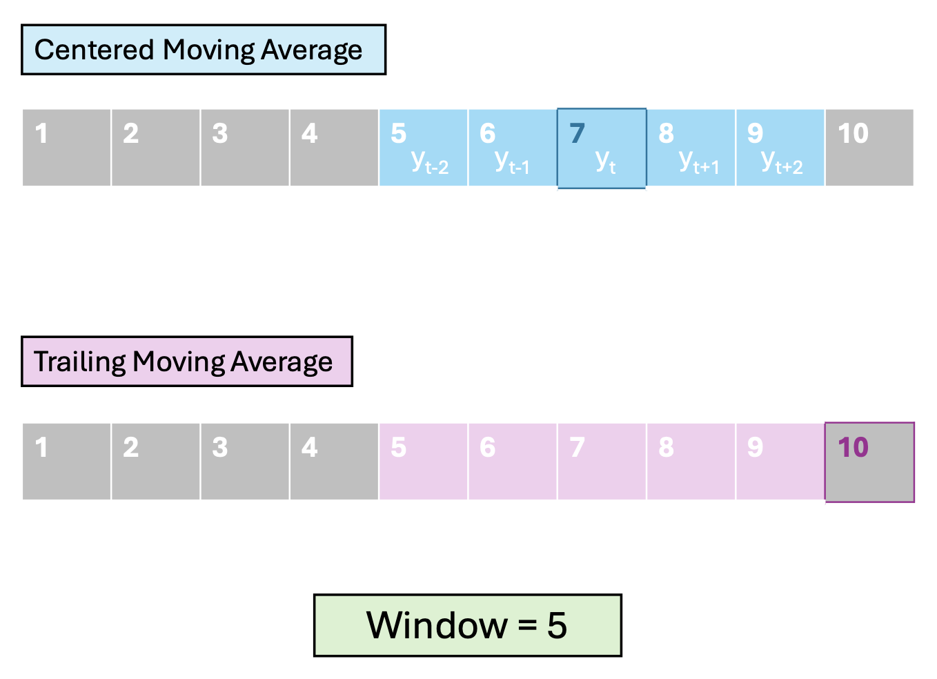
Moving Average (MA) Models
In a MA model, average over a window of consecutive periods.
We define the window by:
width – number of time points
orientation – which time points
It is also possible to weight the time points, e.g., make nearby times more important.
In base R, the filter function gives us an easy way to explore the effect of smoothing.
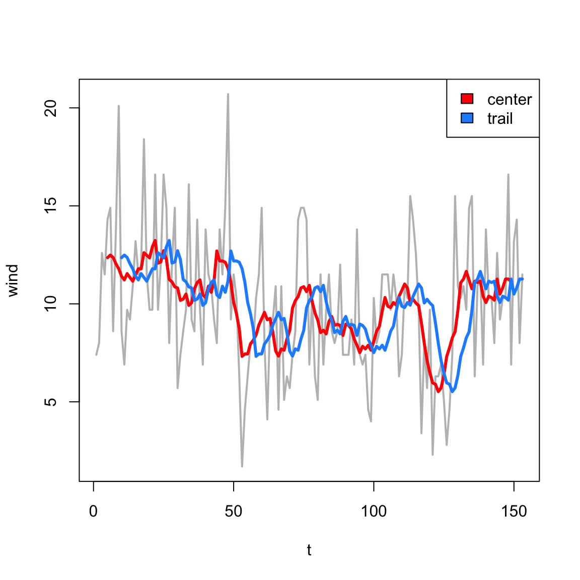
Centered vs. Trailing
t<-1:length(airquality$Temp)wind<-airquality$Wind## centeredFC<-filter(wind, filter =rep(1/9, 9))## trailing: by default## filter function includes point## t in the averageFT<-filter(wind, filter =c(0,rep(1/9, 9)), sides=1)
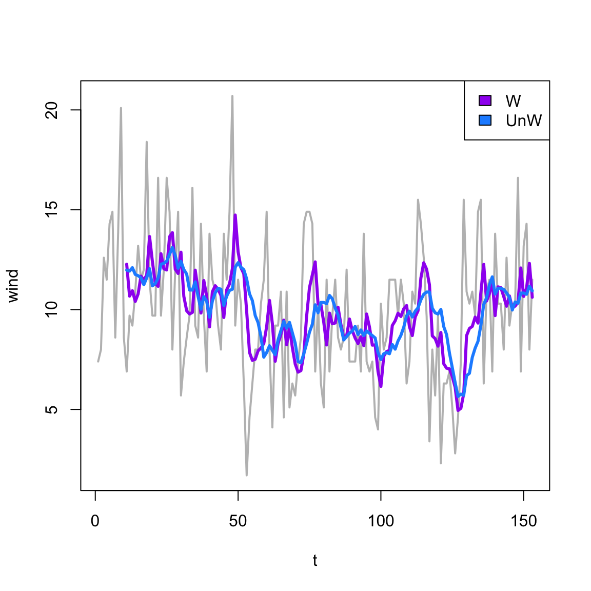
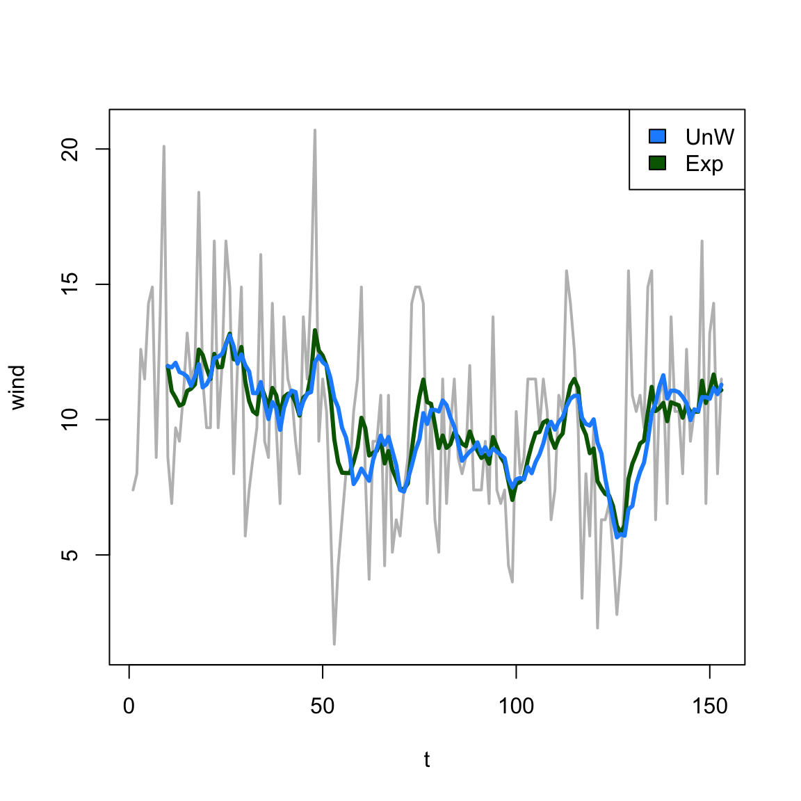
Effects of smoothing: weighting
In base R, the filter function gives us an easy way to explore the effect of smoothing.
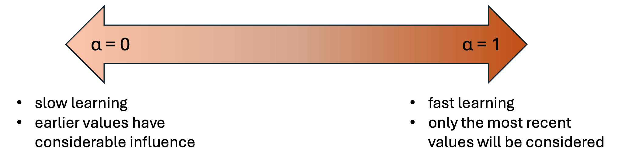
Instead of weighting all points the same, or manually determining weights, Exponential smoothing/moving average (ema) uses a special weighting of \(k\) past values: \[
\begin{align*}
ema_{t+1} = & \alpha y_t + \alpha(1-\alpha)y_{t-1} + \alpha(1-\alpha)^2 y_{t-2} \\
& + \cdots + \alpha(1-\alpha)^k y_{t-k}
\end{align*}
\] where \(\alpha\) is a smoothing constant between 0 and 1. This can be rewritten as a recurssion:
We can combine the idea of smoothing back to capture signal while recognizing the high amount of correlation at nearby time-steps using Auto-Regressive Moving Average (ARMA) models.
We combine the AR(\(p\)) (i.e., using \(p\) lags) with a (trailing) MA(\(q\)) model (i.e., window of size \(q\)).
But how do we build the model?
Specifying the MA part
The tricky bit is that the MA part that goes into the model is not the result of the smoother itself (i.e., it’s not the \(F_t\) on Slide 7).
Instead, we use the residuals – that is, how far the data at the previous time points are from the smoothed estimate based on \(q\) previous times: \[
\varepsilon_{t-1} = y_{t-1} - F_{t-1, q}
\]
ARMA model
The ARMA(\(p,q\)) model is then a regression model (like we saw in our previous AR model) but with extra parameters and terms corresponding to those errors: \[
\begin{align*}
y_t =~& \beta_0 + \beta_1 y_{t-1} + \cdots + \beta_p y_{t-p} \\
& + \varepsilon_t + \theta_1 \varepsilon_{t-1} + \cdots \theta_q \varepsilon_{t-q}
\end{align*}
\]
Pros and Cons of ARMA
Pros:
can capture some signal without needing to specify a functional form
fairly flexible and tunable
Cons:
don’t capture trends or seasonality well (assume nearly stationary)
forecasts must be done one step ahead at a time
ARIMA and SARIMA
In order to relax the assumption of stationarity and allow for seasonality/periodicity, we can add another letter “I” for Integrated and “S” for Seasonal.
What does this mean?
First a digression….
Differencing
AR/ARMA models without explicit trend or periodic components can only describe data that are stationary.
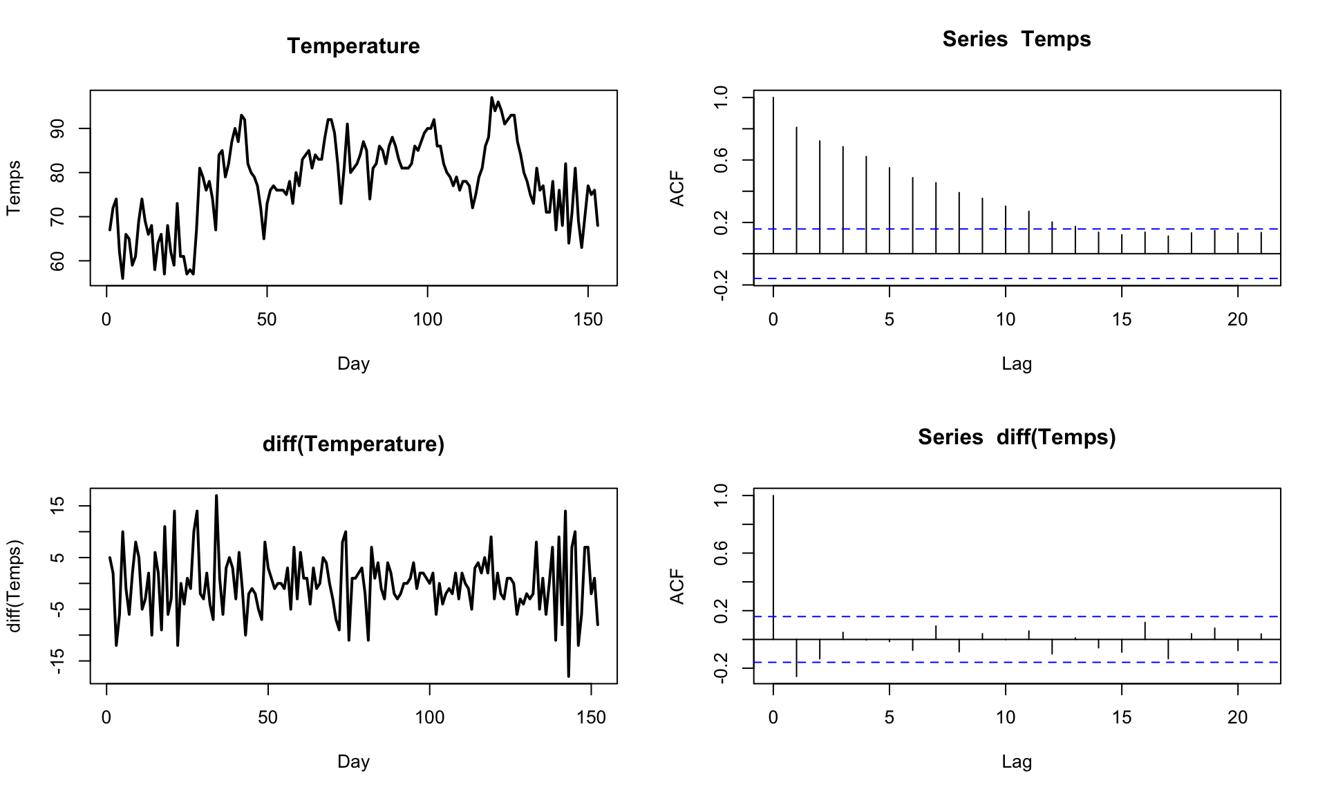
It turns out that we fiddle with a non-stationary TS to get something that is stationary through differencing:
computing the differences between consecutive data points (or at another fixed lag).
Lag-1 differencing removes trends from a TS:
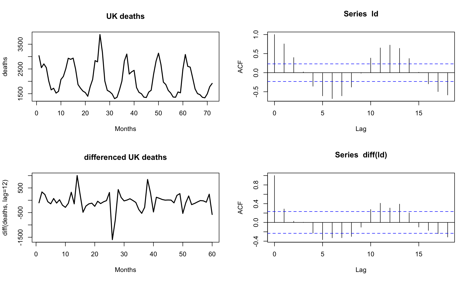
Lag-\(n\) differencing, where \(n\) is the number if steps in a cycle, removes/reduces a seasonal signal from a TS:
back to ARIMA
Now we can get to ARIMA. If we define the Lag-\(d\) differenced time series data as \(y'_t\) then an ARIMA(\(p,d,q\)) model is just:
\[
\begin{align*}
y'_t =~& \beta_0 + \beta_1 y'_{t-1} + \cdots + \beta_p y'_{t-p} \\
& + \varepsilon_t + \theta_1 \varepsilon_{t-1} + \cdots \theta_q \varepsilon_{t-q}
\end{align*}
\] That is, it’s an ARMA model but on the differenced time series to take care of trends.
\(\Rightarrow\) like adding polynomial terms in our regression context.
Fitting an ARIMA model in R
One advantage of ARIMA modeling is that there are automatic ways to choose the order of your model (the \(p, q\), and \(d\)).
This can be convenient when you are only interested in forecasting/prediction.
\(\Rightarrow\) We can use the auto.arima function in the forecast package.
#> Series: ld
#> ARIMA(4,0,1) with non-zero mean
#>
#> Coefficients:
#>          ar1      ar2     ar3      ar4      ma1       mean
#>       1.3183  -0.6933  0.2816  -0.3366  -0.5470  2064.6060
#> s.e.  0.1514   0.2142  0.1946   0.1236   0.1258    37.8362
#>
#> sigma^2 = 93935:  log likelihood = -512.61
#> AIC=1039.21   AICc=1040.96   BIC=1055.15
#>
#> Training set error measures:
#>                   ME   RMSE      MAE       MPE     MAPE      MASE        ACF1
#> Training set 7.15877 293.44 222.1163 -1.384454 10.62095 0.7255362 -0.02699781
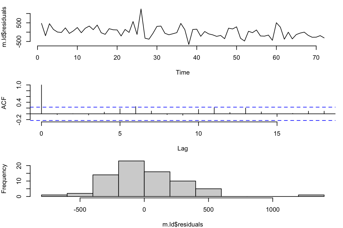
Check the residuals:
One big outlier, but otherwise not too bad
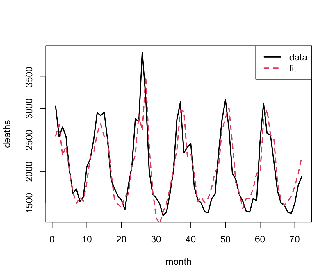
Within-sample predictions:
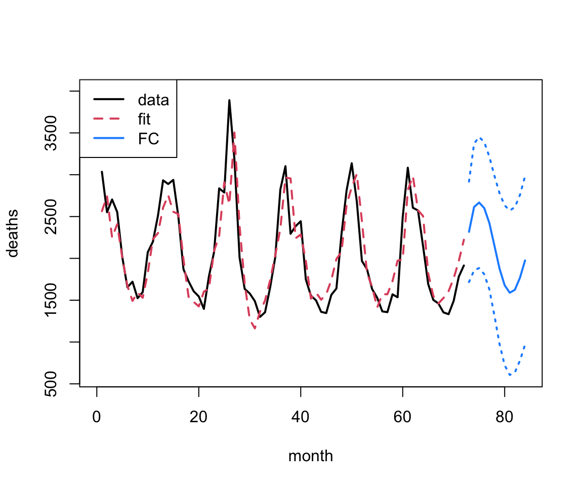
Forecasting
## forecasting at a 12 mo horizonf.ld<-forecast::forecast(m.ld, h=12)
Elaborating on ARIMA
You can include multiple sets of differences in your model.
Specifically, if your differencing reflects the number of time steps over which you observe a periodic pattern, you can add this extra bit on top and create a SARIMA model.
This also requires a second set of variables (\(P,Q\) and \(D\)) to specify what is effectively a second entire model built on the lagged dataset.
Fun trick – AR model of residuals
Let’s say you have time series data, and you had some other model that you wanted to fit – maybe an ODE or even just a smoother.
Often you find that your predictions/forecasts aren’t great because you don’t account for autocorrelation in the error
if you were higher than expected at time \(t-1\) you’re likely to still be a bit high at time \(t\).
How can we incorporate this?
It turns out we can do something really simple to correct for this extra autocorrelation and get better predictions:
Fit the model you want
Fit an AR (or an ARIMA!) model to the residuals
Make the prediction/forecast from these bits together
This works surprisingly well – we’ll see an example of this in the practical.
ARIMA vs. regression approaches
Regression type approaches are highly flexible, and data don’t need to be evenly spaced
lagged predictors can be used as long as the aren’t predictor values missing
Once you add any AR or MA components, or differencing, you must have evenly spaced data w/o gaps
interpreting ARIMA and similar models is tricky – usually they’re better for forecasting
TS analysis is a huge field – we’re only scratching the surface!
Forecasting
We’re going to practice our TS modeling approaches through the lens of forecasting.
That is, we’re going to focus on how to use our TS models to produce a prediction of what we think might happen in the future.
This is actually trickier to do well than you might think…
Recall: Forecasting Process
Define Goal - what to forecast? how far out?
Get Data - what resolution? any predictors?
Explore/Visualize - outliers? spacing?
Pre-Processing - clean and organize data
Partitioning - need to test our forecasts
Modeling - what methods? what predictors?
Evaluation - how good is the forecast?
Implementation - make it repeatable, maybe automate
Evaluating predictions and forecasts
We’ve already learned a few ways to explore how good our model is on the data that we’ve trained it on (within sample).
Mostly we’ve focused on qualitative metrics:
Does the pattern look like the data?
Are there patterns left in the residuals?
Are the residuals still auto-correlated?
Are the residuals normally distributed?
What about quantitative metrics?
Root Mean Squared Error (RMSE)
RMSE is one of the simplest quantitative metrics to calculate: \[
\text{RMSE} = \left(\frac{1}{n}\sum_{i=1}^n (y_i - \hat{y}_i)^2 \right)^{1/2}
\] where \(e_i = y_i - \hat{y}_i\) is the residual for the \(i^{\text{th}}\) data point.
This gives us a quantitative measure of how close, overall, our predictions are to the data.
In-sample vs. Forecasting error
Because RMSE requires that we know the data values, the obvious use is to use it to compare within-sample – fit a couple of models, calculate RMSE, and use it as a tool to decide which model might be better (along with residual diagnostics).
What about forecasting?
If we knew what the future values were going to be, we could also calculate RMSE and compare models!
Data Partitioning
Data partitioning – dividing data into a training set to fit the model and a testing set where we make predictions – is a standard statistical technique.
Often the testing and training sets are divided up randomly (maybe many times) so you don’t accidentally bias your experiment.
However, we cannot remove data at random from a time series as it will impact all aspects of the analysis.
Data Partitioning for Forecasting
When we are dealing with time dependent data, we instead systematically leave out data.
If we have data from times 1 to \(t_{\text{max}}\) we choose a final window of data to leave out:
training: times from 1 to \(t_{\text{test}}\)
testing: times from \(t_{\text{test}}+1\) to \(t_{\text{max}}\)
Then we fit the model just to the training data, make the forecast from the model, and calculate RMSE just on the testing data.
Time Series and Forecasting Practical
In the next practical, we’re going to use our new time series methods on a new data set on tree greenness.
As part of this you’ll practice all of the steps in the forecasting cycle (except the last).